The Problem

Download Data

The powder X-ray Diffraction data is a fast 20 minute continuous scan from 5 to 70 degrees run on a Philips Diffractometer. The reason this data was used was that the sample degraded somewhat by the time a slow Rietveld quality step scan had been run. Rather than twiddle thumbs for the night, it was decided to use the continous scan data. It eventuated that not only could this quick continuous scan data index the phase and assign a space group from the absences; but fitted intensities allowed the structure to be solved with Shelx using Pattersons down to the Oxygens. A new preparation, Rietveld quality XRD data, combined with difference map Fourier contour maps inside the CSRIET software, allowed refinement down to the Lithiums. Neutron data was used to confirm the position and reliability of the Lithium positions.

While the Philips APD 3.6 for DOS software was used for peak profiling on the original structure solution, this goes through the methodology using freely available software.

The scan was collected on a Philips 1710 system with 1050 goniometer (173mm goniometer radius) with Cu LFF X-ray tube at 40mA and 40kV, incident beam Sollers slit with 5.1 degree acceptance angle, no diffracted beam Sollers slit (equivalent of 9.1 degree acceptance angle) 1 degree fixed divergence slit, 0.45mm receiving slit, 1 degree scatter slit, diffracted beam curved graphite monochromator and proportional counter. Continous 20 minute scan from 5 to 70 degrees at 0.025 steps. Slit lengths are 12mm (wide optics) and sample length is ~25mm.

One thing to keep in mind is that some of the misfit could be slight degradation of the sample. Which can make things awkward. Please note that if there is a "new" effect that is not included in the fundamental parameters

Note: Remember that when you add a peak using the fundamental parameters method and XFIT, you have to go back into "File Details, Peaks, Fundamental Parameters Peaks"; change the strain from the default of 0, to match the peaks you are linking this to (or 0.01 if freely refined); change the crystallite size to the peaks you are linking this to; "Use" the peak, then enable the refinement flags for these newly inserted peaks. Tedious compared to the Empirical peak fitting method but such is life.

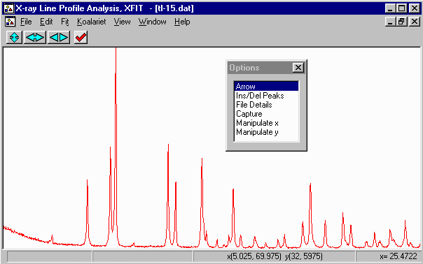
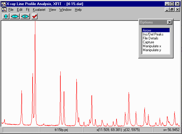
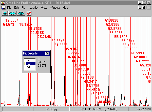
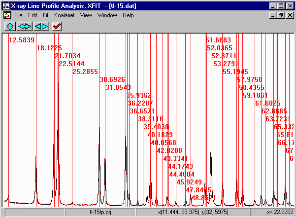
• Run XFIT, (maximise the screen if you wish) and do File, Load Data and open the tl-15.dat dataset. You can maximize the data to fit the entire XFIT screen. It should look something like the following. (if you can't see the active mouse output on the bottom right of the XFIT screen - maximise your XFIT window)

• 

• Examining the data, with fundamental parameters fitting, you should be able to fit the entire pattern. Also, it can be quite tedious zooming and fitting small sub-sections later if the peaks area linked by the same crystallite size and strain code-words. This is because XFIT only refines on peaks visible on the screen; but if linked to peaks outside the screen, things go a bit haywire. Thus if you do zoom up to refine a subset of peaks, you have to make sure any linked parameters are only on the peaks visiible on the screen that you are refining.

Setting up the Cu X-ray Emission Profile, Diffractometer and Background Parameters

• As the characteristic X-rays from the Copper X-ray tube consist of alpha1 and alpha2 wavelengths, the wavelength being used has to be assigned so that the peaks will be profiled correctly.
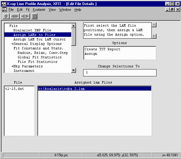
  From the Options box, select File Details elect the Assign LAMs to Files and borwse to c:\koalarie directory and select the cuka_2.lam file.

• 

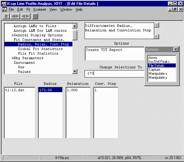
• Go to the Fit Constants and Stats; Radius, Relax Conv.Step and input the goniometer radius of 173mm (highlight the Radius value, type 173 in the "Change Selections To" box and press the ENTER/RETURN key).

• 

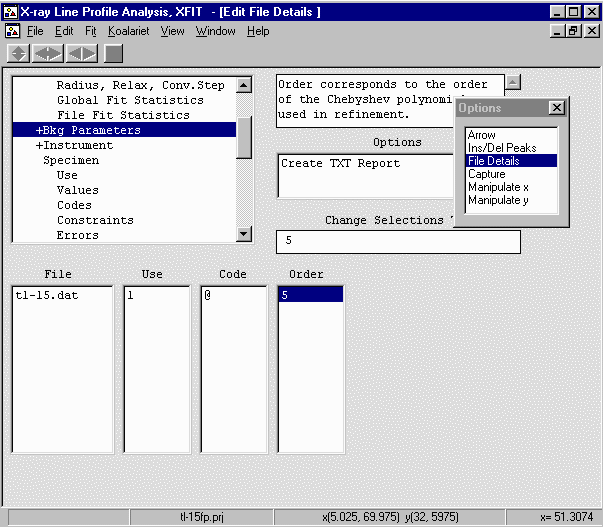
• Continue onto Bkg Parameters and Set the Polynomial order to 5 so it can handle the low angle part of the background.

• 

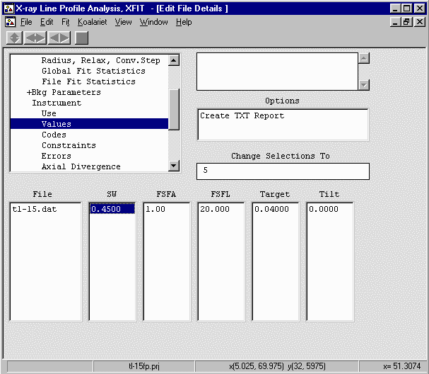
• Continue onto Instrument, Values and set the SW (receiving slit) to 0.45mm, FSFA (Divergence slit) to 1 degree, and X-ray Tube Target (long fine focus) to 0.04mm.

• 

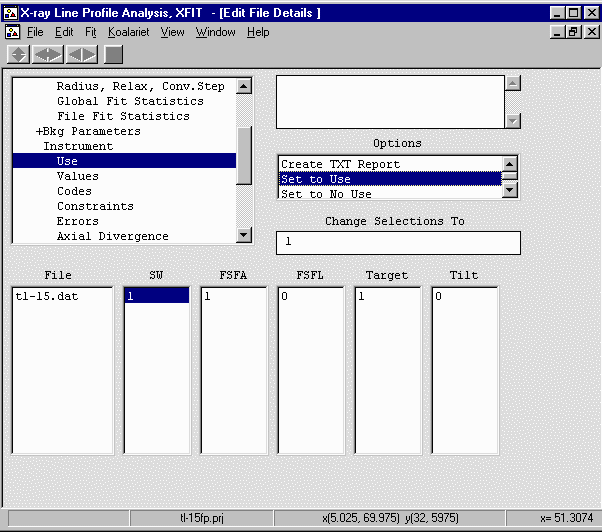
• Go up one to Instrument, Use and enable the above parameters (SW, FSFA, Target) by seleting each 0 value, then Set to Unique Codes from the "Change Selections To" box to convert it to a "1" (Use) value.

• 

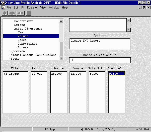
• Go down to Instrument, Axial Divergence, Values and set the Re.Slit (length) to 12mm; Sample (Length) to 25mm; Source (length) to 12mm; Prim.Sol. (Incident Beam Sollers Slit) to 5.1 degree acceptance angle; Scnd.Sol. (Diffracted Beam Sollers Slit) to 9.1 degree acceptance angle which is the same as saying there is no Diffracted Beam Sollers Slit.

• 

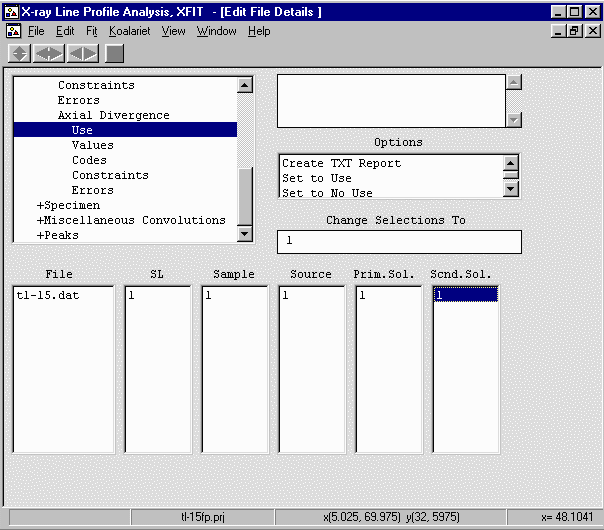
• Go up one to Instrument, Use and enable the above parameters (Re.Slit; Sample; Source; Prim.Sol.; Scnd.Sol.) by seleting each 0 value, then Set to Unique Codes from the "Change Selections To" box to convert it to a "1" (Use) value.

• 

• Congrats! You have setup the machine and background options for this sample. Now it is a matter of inserting, configuring and refining the peaks.

Selecting and Fitting the Peaks

• In the Options box, select arrow use the left mouse key to zoom to 11 degrees and the right mouse button to zoom to 26 degrees. Press s if you miss zoom to get back to the full screen.

• 

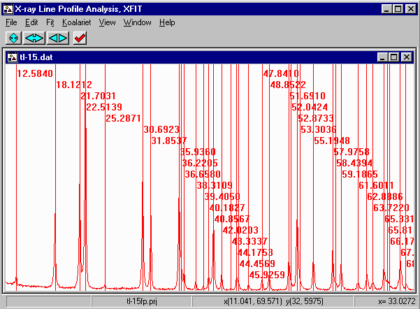
• Select Option, Ins/Del Peaks, Fundamental Parameters Peaks, and insert peaks by clicking the left mouse button.

• 

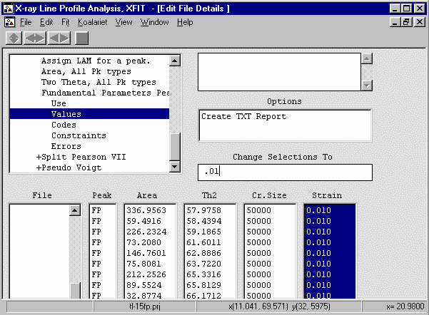
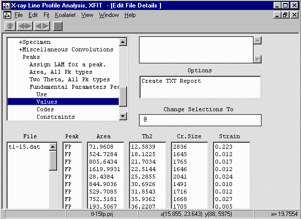
• From the Options box, select File Details, Peaks, Values. Select all the strain value (click and drag) and give the strain values a value greater than zero (i.e., 0.01)

• 

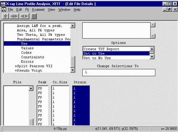
• Go up one menu option to Use and select the Cr Size and Strain values, Set to Use from the "Change Selections To" box to convert it to a "1" (Use) value.

• 

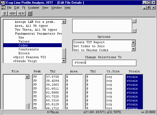
• Go down two menu options to Codes and select the Cr Size and Strain columns, Set the codewords cry and strain in the "Change Selections To" box to convert links the size and strain for all peaks to be identical. The assumption here is that the peaks share identical crystallites size/strain values which may not be the case. The size/strain can be refined individually for each peak. This speeds up the calculation and can result in more reliable values.

• 

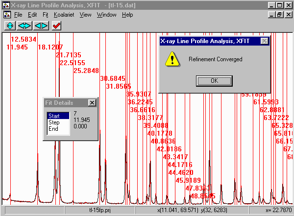
• From the menu select, Fit, Fit Marquardt.

• 

• Then click on start to start fitting and then Yes to keep the refined parameters.

• 

• Note that misfits are due to either problems with the diffractometer system (e.g. misalignment or packing of the sample) , or with the sample, (e.g. more than one peak present, disorder, new/novel form of strain or disorder, degradation of the sample). In this case slow degradation of the sample is the most likely cause of the misfit. It is possible to possibly correct for this by refining various XRD geometry to unreasonable values to some extent; but we will not do this here.

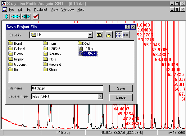
• Just in case XFIT might feel like crashing, save the project file via the menu using File, Save Project As

• 

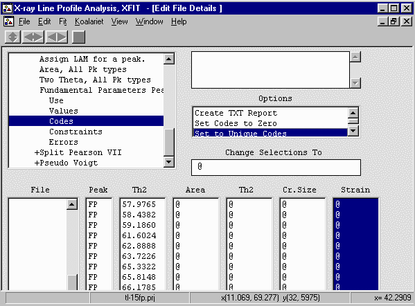
• To freely release the crystallite size and strain to refine for each peak, Options box, select File Details, Peaks, Fundamental Parameters Peaks, Values. Select the Crystallite Size and Strain codewords (cry, strain) and set them to using the Set to Unique Codes

• 

• From the menu select, Fit, Fit Marquardt. Then click on start to start fitting and then Yes to keep the refined parameters. The fit only went down from 11.9 to 11.3 which is not that big a change.

• 

Examining the Peak Fit

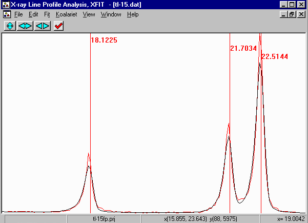
• Zooming up allows you to see the goodness of fit visually. you will note that the fit does not look all that great. This is probably due to degradation of the sample or some form of strain that XFIT is not modelling. Refining on the Sollers slit accpetance angles gives values close to the "official" value for this geometry, implying peak asymmetry is fitting correctly. However, note that a FP fit of the 21.7 and 22.5 peaks imply that the peak inbetween them might be just a bit of noise. The mathematical/empirical fit migth make this situation far more difficult to interpret. Indeed in the Empirical Fitting Using XFIT tutorial - use of an Split Pearson peak shape implied there could be a peak between these two intense peaks.

• 

Obtaining Results

• This results in a list of peaks with ESDs. To generate ESDs, re-fit the range of peaks of interest, then from the menu do Fit, Errors. Go into File Details, Peaks, Fundamental Parameters Peaks, Values, Create Text Report to get the results. Comparing the ESDs with that of the empirical peak fitting on the same sample can be quite revealing; especially the ESDs on FWHM and Shape using Empirical Peak Fitting.

• 

     File        Peak     Area    ESD      Th2      ESD
tl-15.dat       FP      73.7972  7.04     12.5833  0.0152
                FP     525.1695 11.33     18.1219  0.0031 
                FP     808.8842 13.64     21.7033  0.0024
                FP    1617.7630 18.58     22.5138  0.0016
                FP      29.2490  4.03     25.2852  0.0212
                FP     842.7766 13.50     30.6925  0.0022
                FP     530.1695 10.90     31.8536  0.0027 
                FP     755.3265 15.95     35.9364  0.0031 
                FP     194.3486 11.40     36.2205  0.0091 
                FP     135.4252  6.50     36.6579  0.0072
                FP      61.5260  4.51     38.3112  0.0105
                FP      23.0393  3.40     39.4055  0.0230
                FP     115.8754  5.67     40.1829  0.0076
                FP     557.0820 11.02     40.8568  0.0027
                FP     116.2905  5.50     42.0205  0.0069
                FP      12.0952  2.91     43.3329  0.0378
                FP     106.6417  6.94     44.1745  0.0104
                FP      50.8949  6.00     44.4607  0.0192
                FP      43.0744  3.88     45.9254  0.0139   
                FP      81.4082  4.82     47.8408  0.0091 
                FP     126.3955  5.72     48.8521  0.0068
                FP     259.5472  8.78     51.6883  0.0057 
                FP      46.9653  5.74     52.0403  0.0238 
                FP     715.0383 13.28     52.8705  0.0030 
                FP      82.8354  6.46     53.2775  0.0153
                FP     278.5762  8.10     55.1945  0.0045
                FP     333.2409  9.23     57.9765  0.0045
                FP      56.8873  5.20     58.4382  0.0181
                FP     222.0052  7.47     59.1860  0.0054
                FP      69.8183  4.94     61.6024  0.0125
                FP     144.1896  6.40     62.8888  0.0074
                FP      74.4343  5.09     63.7226  0.0128
                FP     212.7719  7.90     65.3322  0.0068
                FP      90.6220  6.80     65.8148  0.0177
                FP      33.6637  5.76     66.1785  0.0374
                FP     301.1027  8.75     67.6631  0.0049    
                FP      47.2308  5.10     68.5051  0.0179