CCP14
Tutorials and Examples
Peak Fitting using Xfit-Koalariet (Coelho and Cheary) for Win95/NT
Empirical Peak Profiling on lab Powder XRD data for Ab-initio Indexing and Structure Solution
The CCP14 Homepage is at http://www.ccp14.ac.uk
[The reference to use for XFIT or FOURYA in any resulting publications is:
Cheary, R. W. & Coelho, A. A. (1996). Programs XFIT and FOURYA, deposited in CCP14 Powder Diffraction Library,
Engineering and Physical Sciences Research Council, Daresbury Laboratory, Warrington, England.
(http://www.ccp14.ac.uk/tutorial/xfit-95/xfit.htm)]
The Problem
Following is a real world example of using Empirical peak profiling and XFIT to obtain
peak information for auto-indexing and structure factor extraction for Patterson based
structure solution. Peak are defined visually. If there is a significant misfit, this could
imply an extra peak is present but care needs to be taken. For difficult problems, indexing
in done iteratively with the peak fitting to check for possible impurity phases.
The data is of a new Lithium Titanate (I.E. Grey, L. M. D. Cranswick, C. Li,
L. A. Bursill, and J. L. Peng, "New Phases Formed in the Li-Ti-O System under
Reducing Conditions", Journal of Solid State Chemistry, 138, 74-86 (1998))
Download Data
Click here to download a zip file of the Liti data
The data is a fast 20 minute continuous scan from 5 to 70 degrees run on a Philips Diffractometer.
The reason this data was used was that the sample degraded somewhat
by the time a slow Rietveld quality step scan had been run. Rather than twiddle
thumbs for the night, it was decided to use the continous scan data. It eventuated
that not only could this quick continuous scan data index the phase and assign a space group
from the absences; but fitted intensities allowed the structure to be solved with Shelx using
Pattersons down to the Oxygens. A new preparation, Rietveld quality XRD data, combined
with difference map Fourier contour maps inside the CSRIET software, allowed refinement
down to the Lithiums. Neutron data was used to confirm the position and reliability of
the Lithium positions.
While the Philips APD 3.6 for DOS software was used for peak profiling on the original
structure solution, this goes through the methodology using freely available software.
The scan was collected on a Philips 1710 system with 1050 goniometer
(173mm goniometer radius) with Cu LFF X-ray tube at 40mA and 40kV,
incident beam Sollers slit with 5.1 degree acceptance angle, no
diffracted beam Sollers
slit (equivalent of 9.1 degree acceptance angle)
1 degree fixed divergence slit, 0.45mm receiving slit, 1 degree
scatter slit, diffracted beam curved graphite monochromator and
proportional counter. Continous 20 minute scan from 5 to 70 degrees
at 0.025 steps. Slit lengths are 12mm (wide optics) and sample
length is ~25mm.
One thing to keep in mind is that some of the misfit could be slight
degradation of the sample. Which can make things awkward.
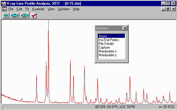
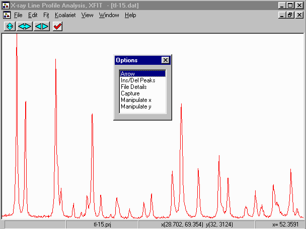
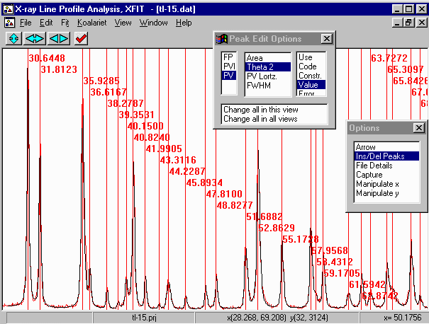
- Run XFIT, (maximise the screen if you wish)
and do File, Load Data and open
the tl-15.dat dataset. You can maximize the data to
fit the entire XFIT screen. It should look something like
the following. (if you can't see the active mouse output on
the bottom right of the XFIT screen - maximise your XFIT
window)

- Examining the data. A personal judgement it that it is probably best to profile the peaks
in two sections; 11 to 26 degrees and 28.7 to 69.4 degrees.
Fitting lower angle peaks
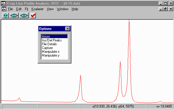
- In the Options box, select arrow use
the left mouse key to zoom to 11 degrees and the right mouse button to zoom to 26
degrees. Press s if you miss zoom to get back to the full screen.

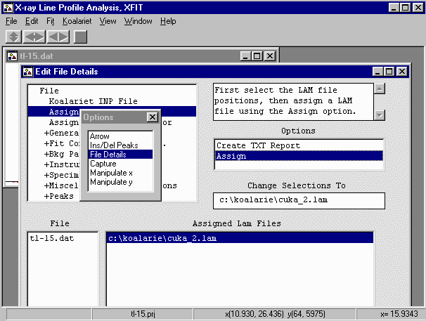
- As the characteristic X-rays have Cuk alpha one and two, we should define this in
the program so that on inserting a peak, both main emissions profiles are modelled.
Go into File Details, Assign LAMs to Files and assign c:\koalarie\cuka_2.lam

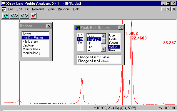
- For these "low" angle peaks, (From the Option, Ins/Del Peaks, PVII)
insert a Split Pearson (PVII) peak to handle the low angle peak asymmetry.
Click left mouse button to add peaks, and right mouse button to delete peaks.

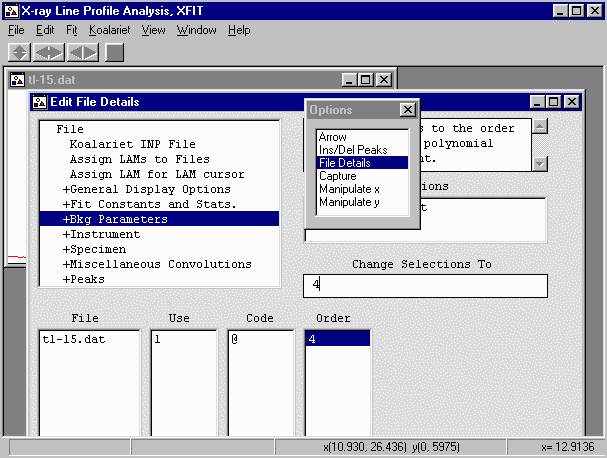
- For the background, Go into File Details and enter a 4th order polynomial to
define the background.

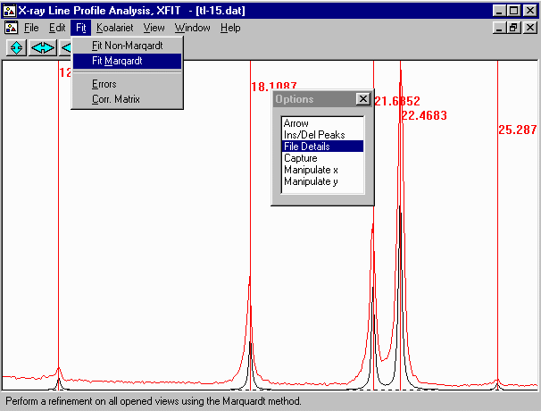
- From the menu select, Fit, Fit Marquardt.

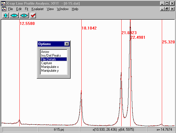
- Then click on start to start fitting and then Yes to keep
the refined parameters. Be wary that a Split Pearson is a very flexible
peak fitting function and it could be modelling two overlapping peaks
as a single peak.

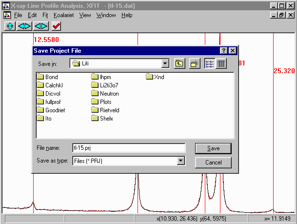
- Just in case XFIT might feel like crashing, save the project file
via the menu using File, Save Project As

Fitting higher angle peaks
- Make sure you have selected the plot window by clicking on it. Press s on
the keyboard to unzoom to view the full data. In the Options box, select arrow
then use the left mouse key to
zoom to ~28.7 degrees and the right mouse button to zoom to ~29.6 degrees. Press s
if you miss zoom to get back to the full screen.

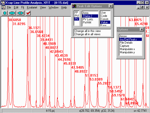
- From the Option, Ins/Del Peaks, PV (Pseudo-Voight), insert symmetrical Psuedo-Voight
peaks. Don't worry if you miss what might be possible peaks as you an insert
them later if there is a decent misfit.
Click left mouse button to add peaks, and right mouse button to delete peaks.

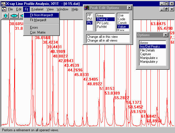
- From the menu select, Fit, Fit Marquardt.

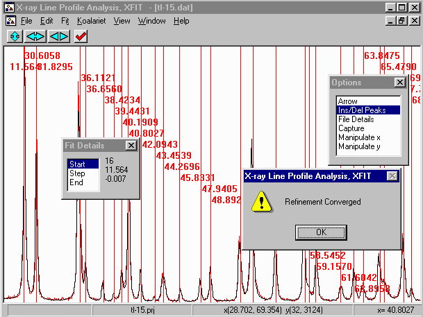
- Then click on start to start fitting and then Yes to keep
the refined parameters. Be wary that even a Pseudo Voight function can be quite
flexible and it could be modelling two overlapping peaks as a single peak.
Arter the refinement converges, click Yes to update the results.

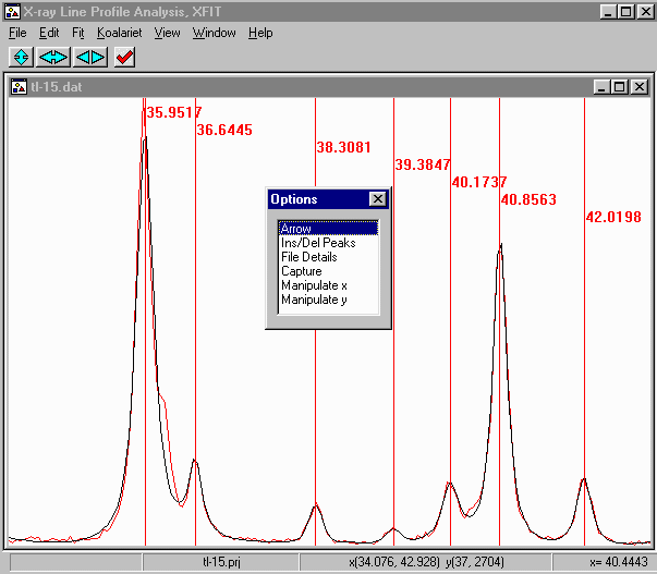
- Misfits could imply other peaks are present or the sample is
degrading. The misfit at 36, sbetween 40.1 and 40.8; and the high angle
end of the 52.86 peak could imply extra peaks. Thus insert extra
peaks here and re-refine. Be careful during the indexing with these
peaks as they may be spurious.

- Here we see a zoomed up portion of the powder XRD pattern with obvious peak misfits.

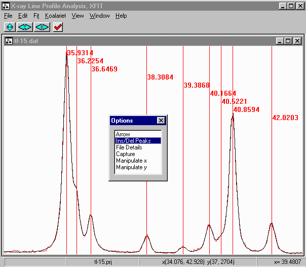
- After fitting two new peaks, the fit below is much better.s

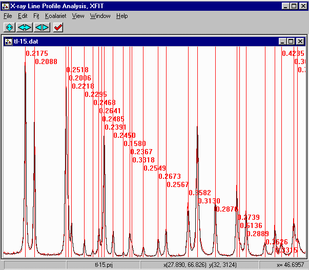
- the next thing to check is how the FWHM (Full Width Half Maximum - Peak Width)
varies. While this could imply peak-asymmetry, FWHM's larger then the average could
be implying there are overlapping peaks. In the Options, Ins/Del Peaks,
Peak Edit Options, select FWHM which displays the FWHM on the screen. Note that the
average FWHM is varying from 0.2 to 0.3. Thus any FWHM outside this range should
be treated with caution as greater than 0.3 could imply overlapping peaks.

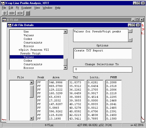
This results in a list of peaks with ESDs. To generate ESS, re-fit the range of peaks
of interest, then from the menu do Fit, Errors. Split Pearson peaks can have
large ESDs on parameters such as peak area, FWHM due to the flexibility and nuances
of this type of peak profile function (e.g., unconstrained peak fitting can give extremely
long tails). Go into File Details, Peaks, (Split Pearson and Psuedo Voight) to get
the results). Note the ESDs on the PVII (Split Pearson) due to unconstrained peak fitting using
this function on small peaks.

     File       Peak     Area      ESD        Th2     ESD
                Type
tl-15.dat       PVII   99.9593       80     12.5525 0.0282
                PVII   588.1507      20     18.1033 0.0068
                PVII  1042.0878     118     21.6934 0.0066
                PVII  1586.0946      27     22.4978 0.0040
                PVII   151.4866    2347     25.3291 0.0279
                PV     930.6631      13     30.6681 0.0017
                PV     548.2765      10     31.8372 0.0020
                PV     863.7153      26     35.9310 0.0033
                PV     129.6226      34     36.2263 0.0102
                PV     158.8826      16     36.6456 0.0078
                PV     65.9024        7     38.3090 0.0072
                PV     20.9200       12     39.3811 0.0168
                PV     46.7854       32     40.1551 0.0097
                PV     122.7227      73     40.4303 0.2552
                PV     542.1722      83     40.8613 0.0026
                PV     123.0962      12     42.0209 0.0054
                PV     13.7453        4     43.3407 0.0187
                PV     92.0356       22     44.1615 0.0200
                PV     84.1511       23     44.4226 0.0489
                PV     49.1961        5     45.9303 0.0102
                PV     90.4678        6     47.8481 0.0072
                PV     144.5448       7     48.8640 0.0055
                PV     294.4215      10     51.7317 0.0044
                PV     763.1232      72     52.8917 0.0048
                PV     119.8731      71     53.2360 0.1763
                PV     305.5976       9     55.2187 0.0037
                PV     333.8850      26     57.9923 0.0064
                PV     79.8515       43     58.3830 0.0529
                PV     259.2144      15     59.2134 0.0051
                PV     91.2168        9     61.6432 0.0104
                PV     164.7747      10     62.9206 0.0064
                PV     87.0643       12     63.7716 0.0119
                PV     147.6010      25     65.3505 0.0091
                PV     249.0785      36     65.8221 0.0425
                PV     365.9529      12     67.7026 0.0048
                PV     34.5275       14     68.5652 0.0162
