[CCP14 Home: (Frames | No Frames)]
CCP14 Mirrors: [UK] | [CA] | [US] | [AU]

(This Webpage Page in No Frames Mode)

[CCP14 Tutorials page] | [Nita Dragoe's Powder for Windows]

Nita Dragoe's Web Site


Let's take the data of NAC available at http://pcb4122.univ-lemans.fr/powdif/low_fwhm_and_rp.html#NAC , in another tutorial by Armel LeBail. The data are in a zip file and some explanations about the conditions used can be seen in the mentioned page. 
Grab the file and unzip it. Before attempting to convert it look at it with an ASCII editor like PFE. We can see some resemblance with the Siemens format but this is not a Siemens format though. We look how many header lines are there (59) and open this file with the program Powder 2.0 with the following options:
-I don't have a header
-Ignore the first 59 lines
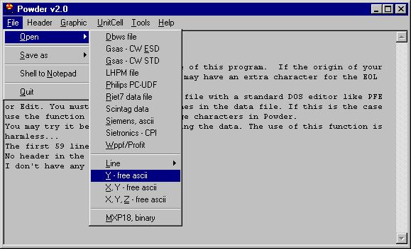
Then open the file as Ascii, and choose the file in question.
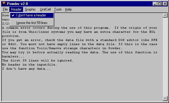
If this is successful you will see some messages (this is what is called Report Pad in this program), in this case what we can see is:

-------------------------------------------------
Y data file, ascii 
The filename is C:\WINDOWS\Desktop\NAC-test-2.UXD
59 line(s) will be ignored.
The number of points is: 6501
Done...
2/15/99 5:26:39 PM
--
NOTE: I have noticed a frequent error in the use of this program. When the data file has been e-mailed without being zipped an extra EOL character appears (I guess it is related to different definition of EOL for DOS and Windows ?). If you look at this kind of file with DOS/Edit you can see alternating empty lines with data. These empty lines will "confuse" the program. Therefore you should remove them by the command Tools/Remove strange characters. The same procedure should be used for files coming from Unix and flavors of Unix.
--

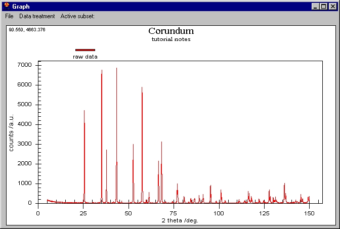
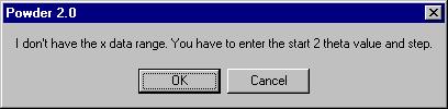
We can directly inspect the data once read by choosing Graphic in the menu. We get this message

and we answer 10 for 2 theta and 0.02 for step (this message comes when the program does not know the starting value and step). Following, the Graphic window is shown:
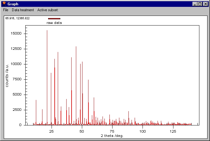
The scale is automatically adjusted to fit all the data. In the top left corner we can see two values 65.916, and 12365...: these are the coordinates of the mouse on the screen. You can roughly inspect the data by this method.
You can zoom as you like by dragging the mouse on the screen:
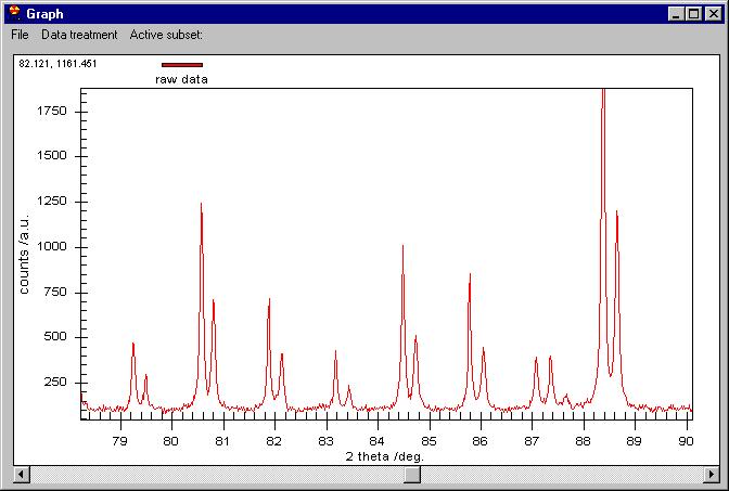
On the zoomed graph a horizontal bar appears. Clicking on it you can move to the right or left by keeping the same zoom as here. You can go back to the initial zoom by right-clicking on the graph area and choosingUndo zoom.
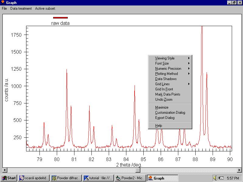
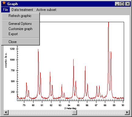
Several other menus are available here, most of them are easy to understand.
When you right-click on the graph an important menu allows changing some parameters:
Note that we can resize the graph at any time. The menu (which can be invoked -for people hating the mouse- by File/General Options command as well) contains:

Viewing style (monochrome or color)
Font size
Numeric precision
Plotting method
Grid lines
Grid in front
Mark data points
Undo zoom
Maximize
Customization dialog
Export dialog
Help

Some of these menus are self explanatory; note that Mark Data Points is extremely slow.
There are two interesting options here: Customization Dialog and Export Dialog, both of them available also from the File menu.

.
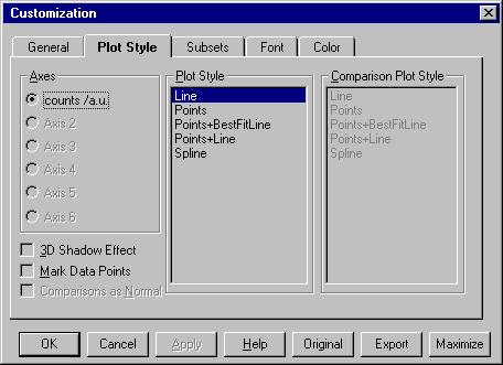
 By Customization Dialog (equivalent with File/Customize Graph) we open the following menu.
The most important command here is Subsets which is described later.

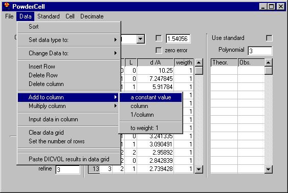
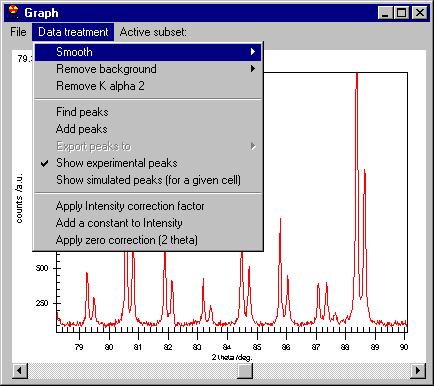
The second menu is Data treatment which allows:
-smooth by Savitzky Golay, Adjacent averaging or a Moving Window algorithm;
-remove background (automatic or manual),
-remove K alpha 2,
-Find peaks,
-Add peaks (not shown here but removing some of the peaks can be done easily, just click on the marker)
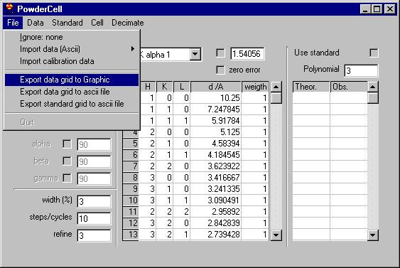
-Export peaks (when you have already determined them)
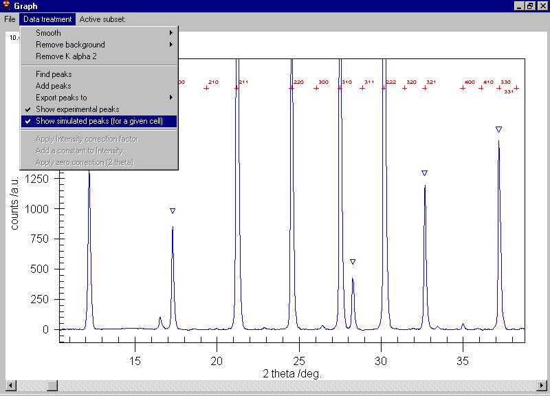
-Show experimental peaks
-Show simulated peaks
-Intensity correction
-zero correction

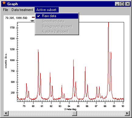
These commands are to be applied to the Active subsets, i.e.
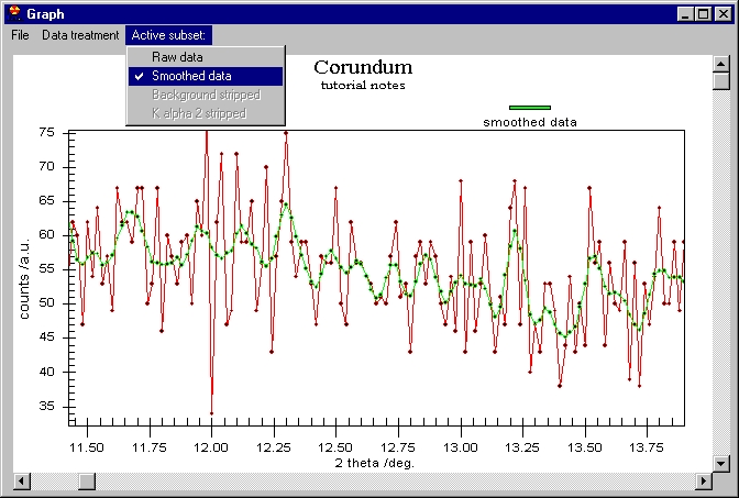
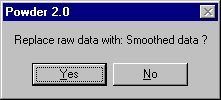
If Active subsets/Raw data menu is checked then smoothing will affect the raw data (Note: you will not loose your original data, all these are applied only in memory). You can smooth the already smoothed data ("massaging" the data if you wish to do so) by checking Active subsets/Smoothed Data.

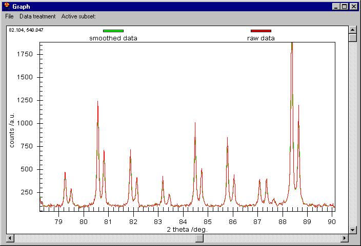
Let's apply smoothing by Data treatment/Smooth/Savitzky Golay method (a parabola through 7 points), after several seconds we get the following screen:

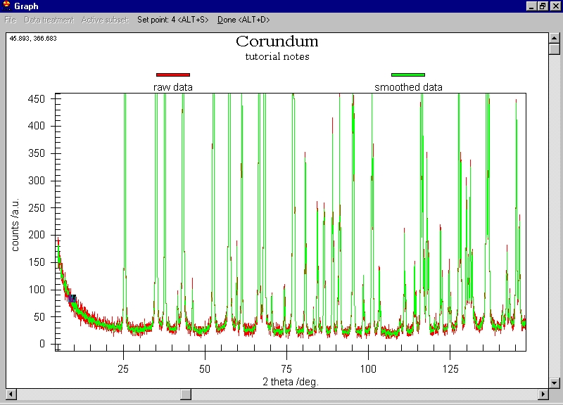
Although it seems that nothing was done, the smoothed data are behind the raw data. You can change this or you can see the difference between the smoothed data and the raw. Note the vertical scroll 
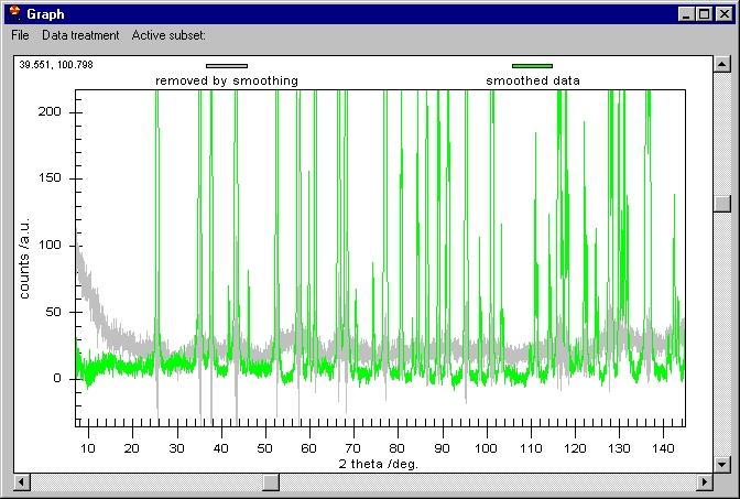
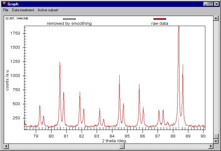
bar here, it is not for zoom but for Scrolling between subsets. If we click 
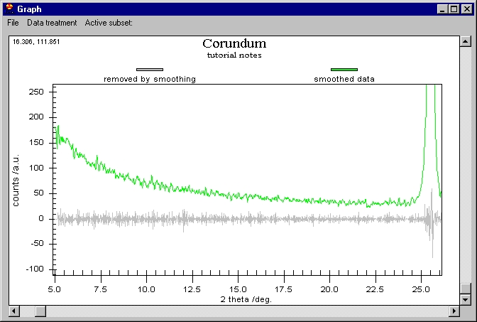
on the vertical scroll bar we obtain this:
The Raw data are kept on the screen but smoothed data have been changed to Removed by Smoothing. The Customization Dialog controls which graph is shown.
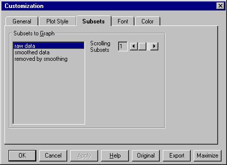
If we go now to Customization Dialog we can see this:
Raw data will be kept on the screen and we can scroll 1 subset. If you select all the subsets or choose Scrolling subsets equal with 2 you will see all the data sets.

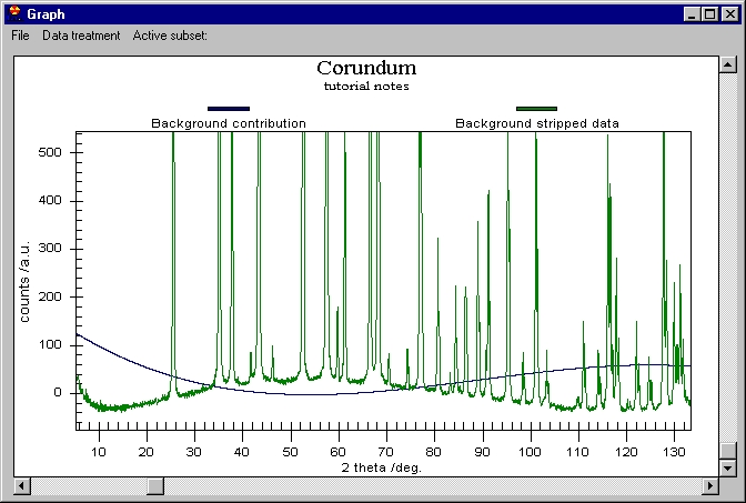
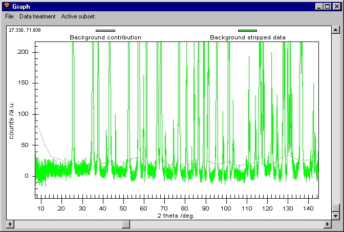
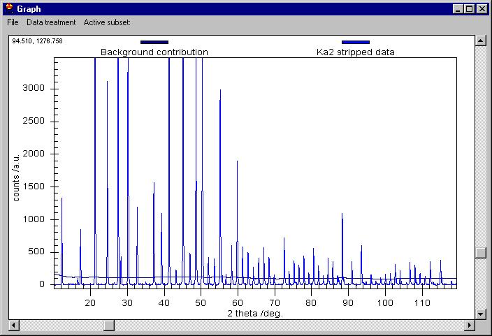
We can now remove the Background (note that Background removal applies to the data which are selected in the Active subset menu) and then K alpha 2 to obtain this:

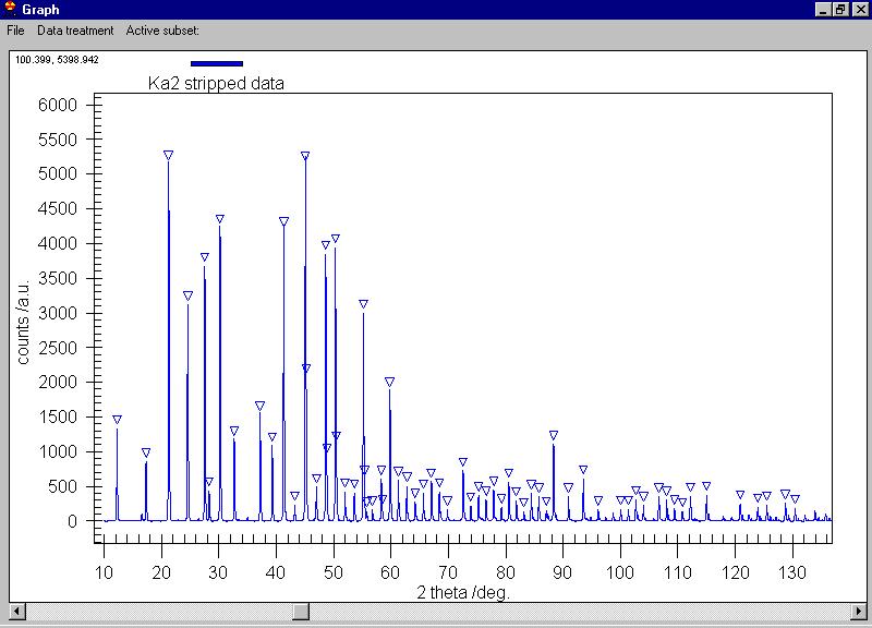
We can search for peaks and the peaks are marked by triangles (some extra peaks appeared, you can delete them by clicking on the triangle)
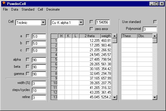
Removing several of the peaks which are obvious due to noise (see the Rachinger method discussion in the book of Klug and Alexander) we can send them all to the data grid, select the Export peaks command:
The values detected are sent to the grid as 2theta and the intensity as weight (the intensity is however ignored hereafter).
You can try to index these by Ito or Dicvol methods. Let's try ITO, select Cell/ Automatic indexing/ Use Ito and the following screen appears:
Only the basic options in ITO can be set up here (NOTE: ITO and DICVOL are independent programs which you should install before using the program Powder. These two well known programs are neither written nor recommended or supported in any way by me!). The data files saved by Powder 2.0 areito.inp and dicvol.inp in the location chosen by Exe location textbox.
In the EXE location field you have to select the location of the program Ito or a directory where the input file ITO.INP should be created when pressing Make file button. You have to go to the DOS end start ITO by yourself.
It gives several solutions (among the suggestions the true solution <much easier to decide when you know the true result, :)>,...)
If you want you can check that one of the solutions is the correct one.
Go to the UnitCell window and enter the value of the unit cell you want to check and the command simulate
The program will compute the theoretical values of 2 theta; select Send DataGrid to Graphic
and these values will be marked with crosses on the graphic. Note: the intensity at which the crosses are put are determined by the value stored in the column Weight. You can easily add a constant to these values
let' say 2000...
Make sure that the menu Show simulated values is checked. You get this kind of figure...
You can print or export this data as you wish.
When exiting the Graphic window, if you want to keep some data (for instance Smoothed data) make sure that the Smoothed data is checked in the Active Subset menu.

You can see 8 graphics at a time (but is difficult to understand them). Let's see corundum (a DBWS file provided by Lachlan Cranswick). We know that is a good DBWS data file so we can read it directly by File/Open/DBWS file from the main part of the program. Then we choose graphic and add a title and subtitle to the graphic. We get this.

We can apply a smooth to this and then check the result (here is shown the smoothed data and what was removed by smoothing).
We should remove the Background now. If the Background is rather small and can be well defined by a low degree polynomial you can apply a Manual Correction (in Remove Background menu). If we want to remove the background of the Smoothed data we should choose Active subsets/Smooth data. In the following figure the Smoothed and Raw data are shown (note the point markers, when showing them be veeeeeery patient).
From now on, as long as the Smoothed Data menu remains checked, all the modifications will be performed on Smoothed data. If you smooth again the old smooth data will be replaced with the new values.

 Manually removing the Background requires choosing some data points. First we should choose the polynomial degree, let's say 3 is enough (the program can accept a degree up to 8 but I do not recommend going to that value). Then we choose data points (the more the merrier) by moving a cursor through points). Choose a point by moving the cursor then Click on Set point or Alt+S to keep the value of the cursor for interpolation. When finished choose Done.

The program will compute the interpolation polynomial based on the values you choose. I selected for this tutorial 12 points and I got this ugly results:
The Background contribution is shown so as you can see what it has computed (this is an example of how should not be the background; you should do better than this).

 Now let's remove the background in a better way (from the raw data, we choose Active Subset/Raw data) and get this.

And now let's smooth the Background removed data (we should chooseActive Subset/Background stripped data) we obtain this:
Note that the Smoothed data contains the Background removed and smoothed data.

If we want to quit the Graphic Window now we will get a message:
That is, if the Active Subset/Smoothed data is checked you will be asked if the data which you read should be replaced by the Smoothed data. If you do not choose an Active subset no matter what modifications you do in the Graphic window the read data will not be replaced.
 

Enjoy and try it extensively to learn how it works.

---
Final note: Remember to register if you'll ever want to ask something or to receive updates and bug reports. If not, you are on your own.
 --
Small print: Use the program at your own risk...

Please contact Nita Dragoe with questions or comments.


[CCP14 Tutorials page] | [Nita Dragoe's Powder for Windows]

[CCP14 Home: (Frames | No Frames)]
CCP14 Mirrors: [UK] | [CA] | [US] | [AU]

(This Webpage Page in No Frames Mode)