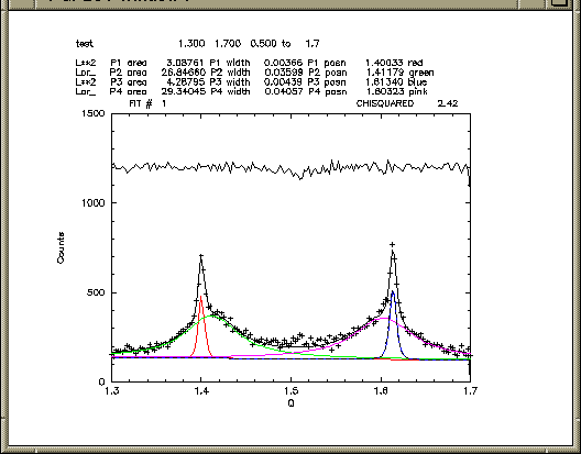
Version 5.4, 6.6, 7.x, 8.0 R.Ghosh, June 2013
This division allows an input routine to be shared amongst a set of similar programs, where the calculation is subject to changes. Similarly the same approach is used in configuring the GUI Clickfit, where help files etc can be shared. A suite of programs for Neutron Reflectometry illustrate well this common usage.
The source is mostly written in standard Fortran77 with timing routines and control-C traps in C. The routines have run on many systems, from DEC-10 (1982) through VMS, SGI, HPUX, Alpha-OSF, linux, and Windows. Current compilations may be found in libraries.
Fitfun allows initial estimates and steps to be set and tried out, using PGPLOT, and then fits data using numerical derivatives with a version of VA05A, a very robust minimisation procedure, which allows a very wide range of problems to be tackled. Each iteration is usually plotted so the convergence can be monitored.
PGPLOT is a general purpose graphics library written by T.J. Pearson from the California Institute of Technology. VA05A is a minimisation routine from the Harwell library written by M.J.D. Powell.
One characteristic of the program suite is the use of the Fortran COMMON to transfer variables internally. This exposes the variables for re-use outside the package, and allows new features to be introduced (e.g. the "4th Column" or error array which is managed by fitfun and also serves to plot error bars in the current (version 8.x) whilst retaining compatibility with versions back to version 6.0.
An additional feature is the inclusion of a dummy subroutine ftextp in the library. If the user programs his own routine it is called by the J command. This routine has often been used, for example, to replot the final fits with overlaying of separately calculated components (passed by Fortran COMMON blocks private to the calculation).
Fitfun_m allows multiple data sets to be fitted simultaneously with parameters either shared or varied individually.
Recent changes
March 2013 (version 8.0)
Data arrays expanded to 21000, Fourth column (e.g.
x-error) values propagated. Error bars may be plotted with command B
[[X] [Y]. Sequence file integrated into main routine; see clickfit. Series of fits may propagate updated
parameters, or re-use initial parameters. Clickfit now includes a command to
interrupt a wildly unstable sequence!
August 2006, version 7.x
New features, primarily the addition of control through a file based
inteface extend the programs through use of a GUI. Clickfit
written using Tcl/Tk is an example, introducing a configurable user interface.
Some new commands have been added, notably simplifying management of
parameters for simultaneous fitting of several sets of data. The treatment
of sequences is now integrated using a control file. The principal
change to help this is the requirement that the READ-IN routine provided
by the programmer now reads the command line left by the R
command. Similarly the J command is also expected to read the
command line. In both cases the command letter has been stripped
before use. This simplifies interaction with the GUI, which
simply has to issue single line commands.
August 2000, version 6.6
To fulfil a need to treat sequences of data a pre-processor stage
has been included in the library, which simplifies the automatic
treatment of sets of data using up to 2 data identifiers (typically
run numbers and subrun numbers). Initially the standard fitfun
is called and a typical set of data are fitted manually. After exiting
this stage the fitted parameters are re-used for a sequence of fits,
eith using the same set of parameters, or using those from the previous
sequence member. More information is given in the
Clickfit description.
The multi-dataset library fitfun 6.1, libffm.a remains unchanged.
September 1999
The version treating one dataset at a time has been extended (v6.2)
to handle 40 parameters. As a consequence for basic use the
NAMEs set in the calling routine /TITLES/ must be extended from 20 to 40.
In internal COMMONs (used by some programs) this change of dimension
affects /CNSTRN/ and /ERRORC/
The current page describes the basic operations in version 6.6.
Working copies of the libraries
may be found in pre-compiled libraries
Versions cover different operating systems
and compilers. Source code and advice on installation and use on
alternative systems may be obtained
from Ron Ghosh,
reghosh (at) gmail.com.
New extensions have been added to fitfun to allow the simultaneous
refinement of several datasets to find an optimum set of model
parameters. This new version (6.0) is still
compatible with single set fits programmed for version 5.4 which
will eventually be phased out of use.
July 1997
Data arrays have been increased to a maximum of 2100 data points.
Exit command now returns to the calling program, with options of skipping reinitialisations and keeping plotting files open. In the latter case the calling program must correctly terminate hardcopy output with CALL PGNEND(2).
In most fitting procedures setting reasonable starting values for parameters is important. By enabling these to be adjusted manually and displaying the model results it is possible to assess the sensitivity of the model to these parameters. This can often offer some physical insight into the problem under study! Initially a subset of parameters can be set with a finite step to allow them to be minimised by the fitting procedure. As convergence approaches additional parameters may be refined simultaneously. In this way rather complex problems may be studied without the fitting procedure becoming unstable or excessively time-consuming.
While it is attractive in terms of cpu time to use analytical derivatives to obtain accurate fits, this can often lead to local minima. Here all derivatives are obtained numerically, and VA05A is usually very good at finding a global minimum. Inevitably if the steps are made very small convergence can require many iterations. Analytical methods can converge very rapidly. Usually, dealing with experimental data, minima are flatter, and a minimum within reasonable experimental error suffices. It is not usually necessary to modify the numerical termination conditions used here (ACC, V 200). It does remain up to the user to play a little with the nominal step sizes for each type of problem. A set of data can then often be treated without futher modifying the steps.
A very simple example is given in appendix I. A more extensive example has also been prepared to show that the routine can be used for routine analysis, by using extensions foreseen in the program, and other routines in the libraries. To this end useful data elements used within FITFUN are identified, and other internal routines are described.

Commands consist of one letter followed by either numerical input (free format) or a letter code (upper or lower case); fields should be separated by blanks or commas. Often the program would be used following the sequence given below.
R [possible input data fields]
The READIN routine is called after this command, and it makes a
new spectrum available to the fitting routine.
D
The current spectrum is plotted.
V
The current variable values are displayed. These are read initially
from a file named "pnam".ffn, where "pnam" is a four character name
defined in the MAIN routine. Parameter numbers 100, 200 and 300
control the fitting procedure (see below) and are not often
modified.
V n v s
The n th variable is set to the value v, and if it is to be fitted
the step s is set to 1. If the model seems very sensitive to this
parameter the value of the step should be reduced to .1 or smaller
and converse. It may be that the model algorithm should be recast.
Normally this should not be necessary. The variation of the n th
parameter can be constrained by being tied to a preceding parameter n'
if s is set to -n'.
X min max
If both min and max are absent or 0 the current spectrum scale limits
are displayed. These may be modified to the new values if these are
none-zero.
Y min max
See above - as for X scale.
F
Without an argument the fit with the current parameters is shown
together with the residual (sum of F(I)**2) normalised by the the
number of points. If the spectrum or fitting range is smaller than
the plotting limits and the Only option has selected a restricted
range then the calculated graph is extrapolated to the plot limits.
(First set the x axis limits, then set the O options). The difference
between the observed and calculated values are displayed offset with
zero at 80% of the yscale limits, with the same scale factors. Adjusting
the y-scale limits may be necessary to reduce overlap with the calculated
curve and data.
P
The fit as given above for F is written out into the second plotting
device defined. Usually this is a PostScript file.
F n [N]
Fitting is started with a maximum limit of n iterations. In general
this should be of the order m**2 where m parameters are being fitted
simultaneously. As fitting proceeds the step lengths for each
variable are also optimised. As a consequence giving a subsequent
F command to continue fitting further iterations resets the step
sizes, and the effect is different from giving a larger total
number initially. If the letter N is added then no intermediate plots will
be made.
L [F]
This produces a summary [or full listing] of the current fit on the terminal
and a file "pnam"xx.lis is produced which may be be printed after
leaving the program.
C
This toggles a cursor on or off for the next D, display command to allow the
current spectrum to be measured-up on-screen.
O a b c d e f
The spectrum is only fitted in the non-zero ranges:
a<x<b, c<x<d, e<x<f
The command O alone resets all points into the range to be fitted.
S
The current parameters are saved in the file "pnam".ffn; this
permits an easy re-use for a subsequent analysis, or simply
to save current values while they are subject to delicate
manual adjustment. (Quit or interrupt program; then restarting will re-read
a saved "good"set of starting values!)
Z
This clears the plotting screen, useful in some terminal environments.
W name
The argument should contain five letters or numbers. The program writes out
the observed and calculated values into a file "name.fpl". The format
of this file is given in appendix 3.
J
The program calls a subroutine FTEXTP (a dummy routine is always
included in the library and is loaded when no personalised routine
is included). This enables the user to perform additional tasks,
e.g. in FIRR and TAPPIR component plots are made of separate
contributions to the resultant curve. The routine can make use of
variables stored in COMMON areas - see the extended example.
T text....
The additional text is placed on the following graphical output.
M seqfilname
seqfilname is the name of a file containing information for treating a
sequence of data; a simple example follows:
 M filseq.fsq

fileseq.fsq:
gtst sequence    title
fitseq.out       output filename (comma separated parameters/deviations for each fit)
T                Reuse first trial (T) or update (U)parameters for next set
50               Number of iterations
r.spc  3.5       input data for each fit as R command
s.spc  4.2                    :
t.spc  4.9                    :
G n1 s n2
Groups stepping of parameter n2 to parameter n1 with step s (This simplifies
establishing links as an alternative to the F command using negative steps).
H
A summary of the above instructions is typed out. If the
programmer has himself provided a subroutine FTXHLP then this
replaces the dummy in the library, and offers a way of adding
further annotation on program use.
	CALL FITFUN (PNAM, READIN, CALSUB)

Input

PNAM    character*4  four characters to be used as the program
                     name to identify the parameter file "PNAM.ffn"
                     and any listing file as "PNAMnn.lis"

READIN               the name of a user supplied routine defined in
                     a Fortran EXTERNAL statement.  This subroutine
                     will be called after each R command to read-in
                     fresh data.  Note COMMONs private to the MAIN
                     and READIN may also be used to store useful
                     data for calculations.  In FIRR, for example
                     numerical resolution spectra are held in this
                     way.

CALSUB               the name of a user supplied routine defined in a
                     Fortran EXTERNAL statement.  This routine is
                     called repeatedly during the fitting procedure
                     to recalculate the model as the parameters are
                     varied.  As indicated above COMMONs may also
                     hold local data values.
MAIN
This serves primarily to provide titles for the parameters to be used
by the fitting routine. The program name PNAM is used to identify
the file "PNAM.ffn" containing saved parameters. It should therefore
only contain alphabetic or numeric characters. It is also used to
generate a systematic listing file name PNAMmm.lis; hence it is useful
to use lowercase letters for PNAM in a Unix environment.
The remaining text fields label the plotting scales and individual variables. The
workspace is set in COMMON/WORK. That shown in the example is adequate
to treat about 128 data varying 10 parameters. It may be expanded
as a first solution should bizarre behaviour be encountered. EXTERNAL
statements are used to allow flexibility in naming subroutines for
reading in data (READIN) and the model fitting function CALSUB.
PNAM, TX and TY and TEXT are all character fields. The labelled
COMMON/VERSION/VERP allows the user to set VERP, a REAL*4 variable,
which may be used to show the program version to the user. The
value of VERP should be less than 100.
READIN
CALL READIN (NPNTS, XOBS, YOBS, YERR, TEXT)

READIN returns
NPNTS     integer*4    the number of points read-in
XOBS)     real*4       arrays of spectrum to be fitted
YOBS)                  observed values, and errors
YERR)
TEXT      character*50 an identifying title
The data arrays are not modified by the fitting routines; subsets of points can be selected ("O" or Only command) feeds a second copy into the fitting routines. Note READIN may have questions within it to slect a part of a larger data-file, and it may also load up private COMMONs to pass other data, e.g. resolution function arrays to the calculation subroutine. Unless the standard library is recompiled the data arrays XOBS,YOBS,YERR should not exceed 2100 elements each.
CALSUB
CALL CALSUB( NPAR,PARM,NFIT,XUSE,YUSE,YRUSE,YCALC,F)

Input
NPAR      integer*4   the number of parameters named in MAIN
PARM      real*4      array of parameters for model
NFIT      integer*4   number of data to fit
XUSE,YUSE, YRUSE  real*4  arrays of preselected data, x values, y
                          and errors in y.

Returned
YCALC     real*4      array of calculated function at each XUSE value
F         real*4      array to be minimised at each XUSE value
The array F will be examined by the fitting routine after each
iteration to find a set of paramters which will minimise the
SUM(F(x)**2). This array might be simply YCALC-YUSE, a function
thereof, or the errors may be introduced as a pre-weighting by
the programmer. Additional data may be introduce via private COMMON blocks.
The YCALC array is used specifically for displaying the function for
direct comparison with the input data. Internal arrays in the calculation
routines should permit 200 points to be calculated (for display and
output purposes). If errors are available (non-zero) then CHI-squared
is calculated.
The parameters can also be used as a simple way of choosing a type of model to be used, by testing it within CALSUB, though clearly the step should then be set always at 0.0!
NOTE:
In programming this calculation routine the programmer must be
aware that values in the X-array XUSE may be incommensurate with
the original data, and that there may be discontinuous steps in
the values. This is of primary importance in performing convolution
fits. Here it is necessary to perform calculations in local arrays,
which cover a range at least equal to that of XUSE values. The results
can then be returned to YCALC by simple linear interpolation, for example,
providing that the local arrays represent the function with a sufficiently
fine mesh. In this type of problem the calculation thus requires:
Problems may arise when the set of parameters are grossly different, e.g. fitting a peak with a half width of 6 channels between channel values 1500 and 1550. Under these circumstances it is clear that the peak position must be varied with a step of 0.001 rather than unity. Often the need to modify the step size should be evident as the initial fits are displayed. Once fitting has started the routine modifies the step sizes used for each parameter. There is consequently a difference between requesting F 25 twice over, and F 50. In the first case the initial step sizes are reset before iterations 26-50, and a 10% (for V 300 0.1) change is re-invoked before the second go at fitting.
At the expense of requiring many more iterations the value of the general SUBSTEP may be reduced when the model appears overly sensitive (e.g. set V 300 0.02 for a 2% initial shift). Inspection of the modified parameters (V) will also show-up cases where the individual parameter's step has been set too small such that modifying it has no appreciable effect on the residual sum. If, after a few iterations extending the step by small amounts there is still no effect then no further changes are attempted.
The final accuracy to attain for termination is controlled by ACC (parameter 200); this is estimated as ACC*0.001*(initial residual value).
If no improvement to the fit arises due to the sizes of these initial steps the routine will fail to advance. Reduce the steps for obviously oversensitive parameters, or recast the calculation.
No minimum is also signalled when after proceeding through a number of iterations shows no improvement greater than the termination condition. Often by this stage the results are acceptable, within the limitations of the data.
One further fitting control is DMAX (paramter 100), which is a metrix of the total change in parameters. This is normally set to 100, and is rarely changed, so it is reset to this value by the program on starting, and is not conserved in the parameter file.
The deviations and the covariance matrix are only evaluated correctly at the minimum. Values in the covariance matrix less than about 20% may be considered as being subject to large errors, bur indicate that there is no significant parameter correlation. This may be expected when off-diagonal terms exceed 50%.
at present the routines are compiled with limits of a maximum of 40 named parameters, with data arrays limited to 21000 elements. VA05A requires a workspace array which is defined in the MAIN program and should not be less than that shown in the example. Use with more parameters or larger data fields require modification of the source code and recompiling. If problems related to overwriting the workspace are evident then COMMON/WORK/SPACE(3000000) should be increased as a first attempt to resolve the error.
Units 1 and 2 are used for internal file-handling.
Unit 16 is used for the listing file output.
Units 5,6 are used for terminal input and output respectively.
The program must be loaded with the ILL PGPLOT library, (Unix,PC, OpenVMS) together with the X11 library (Unix). One simple way of identifying the libraries simply is to create a link in the local directory for each library file
(e.g. linux)
ln -s ../libsLgf/libffn74lgf.a libfitfun.a
ln -s ../libsLgf/libpgplot.a libpgplot.a


the program is then linked as follows:
(linux)
gfortran -o myprog myprog.f myread.f mycalc.f libfitfun.a libpgplot.a /usr/X11R6/libX11.a
(os x)
gfortran -o myprog myprog.f myread.f mycalf.f libfitfun.a libpgplot.a
/usr/X11R6/libX11.6.dylib
for MinGW (PCs)
g77 -o myprog myprog.f myread.f mycalc.f libffn70m.a libpggw520.a -mconsole -mwindows
These are for the plotting library. The graphs expect a form with a width/height aspect ratio of 4:3 For A4 output in PostScript Landscape layout (/CPS) should be chosen for one graph per page. In the examples below two pictures per page are set, with portrait mode selected.
for linux
% setenv PGPLOT_DIR ../libsLgf
%# directory containing font file etc.
% setenv PGPLOT_ILL_DEV_1 /XSERV
%#X server - pgxwin_server
% setenv PGPLOT_ILL_DEV_2 /VCPS
%#Colour PostScript hardcopy - portrait format
% setenv PGPLOT_ILL_PPAGE 2
%# two pictures per page


and for PCs
c:>SET PGPLOT_DIR=C:/libm
C:>SET PGPLOT_ILL_DEV_1=/GW
C:>SET PGPLOT_ILL_DEV_2=/VCPS
General Information on building programs using these ibraries is shown in tha adjacent link
Other programs using fitfun
Neutron Reflectometry by Professor Rennie SANS - functioning examples in SANS distributions SANS - peak fitting sasfit4 SANS - model fitting polymer SANS - spherical shells - ssqfun SANS - eleven model functions - rfit SANS - scattering and secondary scattering from hard spheres - hs2 ToF - inelastic/quasi-elastic peaks - convolutions FIRR Diffraction peak fitting sequences etc. f24s etc.This simple program reads a formatted data file and fits a Gaussian curve with a sloping background.
Main Program
PROGRAM FTEST C***** BASIC EXAMPLE ROUTINE FOR FITFUN C***** Link FTEST,MYREAD,GAUSS,FITFUN/LIB,LIBPG/LIB C HP setenv LPATH /lib:/usr/lib:/usr/local/lib:/usr/lib/X11R5 C HP f77 -o ftst ftst.o myread.o gauss.o libfitfun.a -lpgplot -lX11 -lU77 C IRIX f77 -o ftst ftst.o myread.o gauss.o libfitfun.a libpgplot.a -lX11 C EXTERNAL MYREAD,GAUSS C C***** MYREAD IS A USER SUPPLIED ROUTINE TO READ IN ONE SPECTRUM EACH CALL C C***** GAUSS IS A USER'S ROUTINE TO CALCULATE THE REQUIRED FUNCTION C COMMON/TITLES/NAMES(40),TX,TY COMMON/TITLEP/NPARAS COMMON/WORK/W(3000000) C***** THIS IS SUFFICIENT FOR 21000 DATA AND 40 PARAMETERS ! COMMON/VERSION/VERP C***** VERP IS TYPED BY THE PROGRAM INDICATING THE CURRENTLY RUNNING VERSION C CHARACTER*8 NAMES CHARACTER*4 PNAM CHARACTER*20 TX,TY C DATA NAMES/'Centre ','Sigma','Flat Bkd','Slope', 1'Height',35*' '/ DATA PNAM/'ftst'/ DATA TX/'Channel'/ DATA TY/'Counts'/ DATA NPARAS/5/ C VERP=3.1 C***** Sets a version for fitfuns to print out as identification WRITE(6,1) VERP 1 FORMAT(' FTST - Simple Demonstration program for Fitfun'// 1' Version ',F4.1,' August 1999 (REG)'/) C***** SIGNIFIES THIS IS VERSION 3.0 of FTEST CALL PRELUDE(PNAM) C***** (optional) initiates interface for use with clickfit gui CALL FITFUN(PNAM,MYREAD,GAUSS) c***** this is where it all happens! C END SUBROUTINE FTXHLP(IOTTY) COMMON/VERSION/VERP WRITE(6,1) VERP 1 FORMAT(' FTST - Simple Demonstration program for Fitfun'// 1' Version ',F4.1,' August 1999 (REG)'/) RETURN ENDRead-in routineSUBROUTINE MYREAD(NPNTS,XOBS,YOBS,YERR,NTEXT) c***** uses command line input c..... GUI error out COMMON/TINC/PNAM,RET80 COMMON/REPLY/RESOUT DIMENSION XOBS(*),YOBS(*),YERR(*) CHARACTER*50 NTEXT CHARACTER*20 FNAME CHARACTER LINE*80,LINED*81 CHARACTER PNAM*4,RET80*80,RESOUT*80 EQUIVALENCE (LINE,LINED) LINED(81:81)='/' 10 NPNTS=0 READ(RET80,*) FNAME 2 FORMAT(A) c FNAME=RET80 OPEN(UNIT=10,FILE=FNAME,ACCESS='SEQUENTIAL',STATUS='OLD',ERR=99) C***** NOTE UNIT IS NOT 1 C***** SIMPLY FORMATTED FILE READ(10,3,ERR=99,END=99) NTEXT 3 FORMAT(A) C***** THIS CAN SERVE AS A TITLE FOR THE SPECTRUM DO 5 I=1,180 READ(10,6,END=99) LINE READ(LINED,*) XOBS(I),YOBS(I),YERR(I) C***** PICKS EITHER 2 OR 3 VALUES PER LINE 6 FORMAT(A) NPNTS=I 5 CONTINUE 99 CLOSE(UNIT=10) IF(NPNTS.LE.5) GO TO 12 WRITE(6,9) NTEXT 9 FORMAT(' TITLE: ',A/) WRITE(6,11) NPNTS WRITE(RESOUT,11) NPNTS 11 FORMAT(1X,I4,' DATA HAVE BEEN READ IN') 1111 RETURN 12 WRITE(6,98) 98 FORMAT(' INSUFFICIENT DATA TO CONTINUE') C***** DO NOT RETURN UNTIL SOME GOOD DATA ARE READ RESOUT='ERR: INSUFFICIENT DATA TO CONTINUE' GO TO 1111 ENDCalculation routineSUBROUTINE GAUSS(NPAR,PARM,NFIT,XUSE,YUSE,YRUSE,YCALC,F) C C Calculation of F and YCALC for gaussian C DIMENSION PARM(NPAR) DIMENSION YCALC(NFIT),XUSE(NFIT),YUSE(NFIT) 1,YRUSE(NFIT),F(NFIT) C C DO 10 I=1,NFIT C***** YCALC will contain calculated function for plotting/listing YCALC(I)= PARM(5) * 1 EXP(-0.5*((XUSE(I)-PARM(1))/PARM(2))**2) 1 +PARM(3) + PARM(4)*XUSE(I) F(I)=YCALC(I)-YUSE(I) C***** F will be minimised by VA05A; no weighting is used here 10 CONTINUE C C RETURN ENDA small test data set, test.dat, follows:TOF data at 1.5K 300.0 28.00 5.29 301.0 19.00 4.34 302.0 9.000 3.00 303.0 28.00 5.29 304.0 31.00 5.57 305.0 30.00 5.48 306.0 50.00 7.07 307.0 82.00 9.06 308.0 92.00 9.59 309.0 277.0 16.64 310.0 882.0 29.70 311.0 2573. 50.72 312.0 5164. 71.86 313.0 7586. 87.10 314.0 8238. 90.76 315.0 6453. 80.33 316.0 3663. 60.52 317.0 1473. 38.38 318.0 450.0 21.21 319.0 128.0 11.31 320.0 68.00 8.25 321.0 53.00 7.28 322.0 34.00 5.83 323.0 33.00 5.74 324.0 24.00 4.90 325.0 24.00 4.90As an exercise the starting values should be entered manually. Below is a copy of typical values which have been stored in ftst.ffnftst V 3.1 using FITFUN V 7.0 12-Aug-2006 16:10:26 0.05 0.1000E-01 H(Substep), ACC 0.0000E+00 0.0000E+00 FITTING LIMITS 0.0000E+00 0.0000E+00 FITTING LIMITS 0.0000E+00 0.0000E+00 FITTING LIMITS 300.0 350.0 X PLOTTING LIMITS 0.0000E+00 0.1200E+05 Y PLOTTING LIMITS 311.0 0.0100 CENTRE 2.000 0.1000 SIGMA 30.00 1.000 FLAT BAK 0.0000E+00 0.0000E+00 SLOPE 8000. 1.000 HEIGHTA Script for the test session follows:is1 146% ftst ftst version 3.1 TYPE HELP OR OPTION: H,R,D,X,Y,V,F,O,P,L,W,C,E,J,S,T,Z ftst>r test.dat TITLE: TOF data at 1.5K 26 DATA HAVE BEEN READ IN THERE ARE 26 DATA POINTS IN CURRENT FITTING RANGE TYPE HELP OR OPTION: H,R,D,X,Y,V,F,O,P,L,W,C,E,J,S,T,M,G,Z ftst>v FITFUN 7.0 TITLE: TOF data at 1.5K FITTING Y : COUNTS VERSUS X : CHANNEL NUMBER PARAMETER VALUE ( OLD VALUE ) STEP % DEVIATION 1 CENTRE 311.0 ( 311.0 ) 0.1000E-01 0.0 2 SIGMA 2.000 ( 2.000 ) 0.1000 0.0 3 FLAT BAK 30.00 ( 30.00 ) 1.000 0.0 4 SLOPE 0.0000E+00( 0.0000E+00) 0.0000E+00 0.0 5 HEIGHT 8000. ( 8000. ) 1.000 0.0 100 MAXIMUM STEP 100.0 300 SUBSTEP 0.05000 200 ACCURACY 0.1000E-01 THERE ARE 26 POINTS IN THE CURRENT RANGE SET BY "ONLY" COMMAND. CURRENT LIMITS (IF RANGE IS NON-ZERO) ARE : 0.000E+00 TO 0.000E+00 0.000E+00 TO 0.000E+00 0.000E+00 TO 0.000E+00 TYPE HELP OR OPTION: H,R,D,X,Y,V,F,O,P,L,W,C,E,J,S,T,M,G,Z ftst>f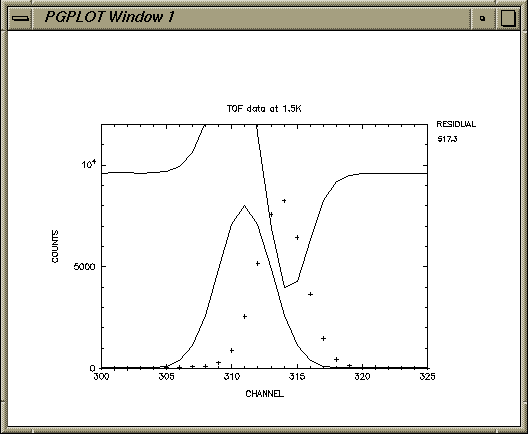 TYPE HELP OR OPTION: H,R,D,X,Y,V,F,O,P,L,W,C,E,J,S,T,M,G,Z ftst>f 100 FITTING..... .....ENDED
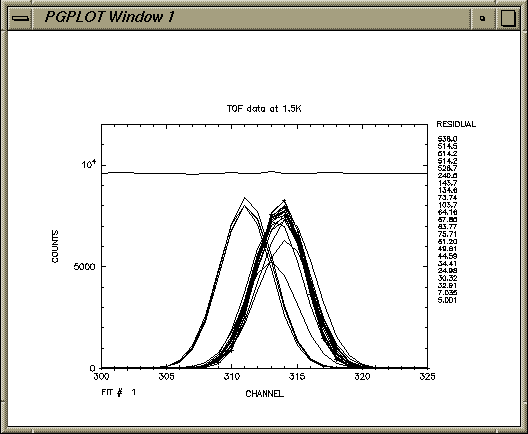 TYPE HELP OR OPTION: H,R,D,X,Y,V,F,O,P,L,W,C,E,J,S,T,M,G,Z ftst>f
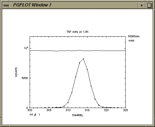
TYPE HELP OR OPTION: H,R,D,X,Y,V,F,O,P,L,W,C,E,J,S,T,M,G,Z ftst>p TYPE HELP OR OPTION: H,R,D,X,Y,V,F,O,P,L,W,C,E,J,S,T,M,G,Z ftst>l FITFUN 7.0 TITLE: TOF data at 1.5K FITTING Y : COUNTS FIT NUMBER 1 VERSUS X : CHANNEL NUMBER PARAMETER VALUE ( OLD VALUE ) STEP % DEVIATION 1 CENTRE 313.7 ( 311.0 ) 0.1000E-01 0.0 2 SIGMA 1.762 ( 2.000 ) 0.1000 0.2 3 FLAT BAK 28.53 ( 30.00 ) 1.000 18.6 4 SLOPE 0.0000E+00( 0.0000E+00) 0.0000E+00 0.0 5 HEIGHT 8304. ( 8000. ) 1.000 0.2 100 MAXIMUM STEP 100.0 SUBSTEP 0.05000 200 ACCURACY 0.1000E-01 CURRENT RESIDUAL VALUE : 4.8100 THERE ARE 26 POINTS IN THE CURRENT RANGE SET BY "ONLY" COMMAND. CURRENT LIMITS (IF RANGE IS NON-ZERO) ARE : 0.000E+00 TO 0.000E+00 0.000E+00 TO 0.000E+00 0.000E+00 TO 0.000E+00 Mean R-factor is now 23. % (old value 0.00E+00%) Reduced CHI-squared is now 5.3 for 22 degrees of freedom (old value 0.00E+00) Chi-squared probability is 0.640E-14 TYPE HELP OR OPTION: H,R,D,X,Y,V,F,O,P,L,W,C,E,J,S,T,M,G,Z ftst>e DO YOU WISH TO SAVE THE CURRENT PARAMETER VALUES ? (Y) n Closing listing file ftst068.lis %PGPLOT, Completing PostScript file ftst067.ps is1 147% lp ftst067.ps is1 148% lp ftst068.lisAlthough the fit looks impeccable, the chi-squared is quite large. If the final graph is rescaled, giving the commandsTYPE HELP OR OPTION: H,R,D,X,Y,V,F,O,P,L,W,C,E,J,S,T,M,G,Z ftst>y 0 500 TYPE HELP OR OPTION: H,R,D,X,Y,V,F,O,P,L,W,C,E,J,S,T,M,G,Z ftst>fit is then possible to see that there is a marked discrepancy between the simplistic model and the real data, which is reflected in both the R factor and Chi-squared.