Using the six-position sample changer

The six-position sample changer can be used to collect room temperature data on up to six different samples under control of the data collection program, ICP. The steps to be followed for automatic usage are outlined below and then will be discussed subsequently in more detail. Note that the function key references (e.g. F17) refer to the labels on the console computer, not to the the letters on the keys.

Summary of steps

1.

Mount the sample changer and connect the motor controller.

2.

Ensure the changer works and the correct sample is rotated into position (NEXT).

3.

Define parameters for run in ``Prepare mode.''

4.

Set the data collection time using Automon.

5.

Copy and edit the parameters for additional runs.

6.

Set up a run sequence (RS=...).

7.

Switch to control mode (F17) and check the run sequence timing (HOWLONG/RS).

8.

Check and log the neutron monitor (MRAT) as well as document the sample on: a sample tag, the white board and in the log book.

9.

Start the run sequence (RS).

Detailed discussion

1.

Physically move the sample changer into position and connect the two motor controller cables marked ``Sample Changer'' A and B. They are polarized so that they can only be connected in one way.

2.

Load your samples into the changer, paying careful attention to the position number of each sample. A good practice is to fill out a sample tag for each sample before you load the samples and then mark down the position number on the sample tag.

3.

Check that the sample changer advances properly by typing NEXT. Note that it takes about 1 minute for the sample changer to completely advance and the Motor 15 display to be set correctly. If the display is not correctly synchronized with the actual position, the display can be reset using the INI15=# command, where # is 1,2,3,4,5 or 6.

4.

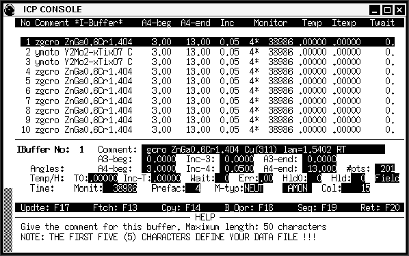
In ``Prepare Mode,'' define a run to be measured in what is called an ``increment buffer'' (see Figure 14). Each ``buffer'' line defines the parameters for a single diffactometer scan. For convenience, you may wish to use the buffer numbers that correspond to the positions of your samples in the sample changer.

  

Figure 14: Defining a single run in ``Prepare Mode.''

For use with the sample changer, a temperature controller, you will typically need to set the following fields in the buffer: Comment, T0, Monit, Prefac. and M-typ, which are used as follows:

Comment

This sets a 1-line file header and the name of the data collection file. Be sure to use letters and numbers (A-Z and 0-9) and no other characters for the first five letters of the Comment as this is used for the file name. If an invalid name is used the file will be named DEFLTxxx.BT1, where xxx is a number in the range 001 to 999.

T0

This specifies the nominal temperature for data collection. T0 should be 0, when temperature control is not being used. This causes the Wait, Err, Inc-T, and Hld0 values to be ignored.

M-typ

Is either ``NEUT'' or ``TIME''. NEUT is used for most data collection, where the data collection time is adjusted to match the neutron flux on the sample.

Prefac

Each data point is measured ``Prefac'' times and if Prefac is 4 or greater, the measurements are checked for statistical agreement, so that significant noise spikes can be discarded. A rule of thumb is that Prefac should be 4 for runs of 6 hours or less. It may be desirable to increase Prefac by 1 for each additional 6 hours of length, but 4 is a good default value regardless of the data collection time.

Monit

This value, along with Prefac, determines the length of the data collection period. If M-typ=TIME, this specifes a count time in seconds. Most commonly, M-typ=NEUT and Monit is set using the AUTOMON (AMON) feature.

It is very unlikely that you will want change the default values for some fields: A3-beg, A3-end, Inc-3, A4-beg, A4-end, Inc-4 and #pts. The Col field informs ICP of the in-pile collimation (15' or 7'). The default, 15' is usually correct. Note that the A4-*, #pts and Col values are reset every time a buffer is edited. There is one exception to this. If you are setting up runs while the instrument is collecting data and plan to use a different monochromator than the one that is currently in use, you may need to change the A4-beg and A4-end values to match the monochromator you plan to use. Use 3-13 degrees for Cu311 and Si531 and 1.3-11.3 degrees for Ge311. Note that the A- command in control mode turns off the automatic resetting of A4-beg and A4-end.

Note that the field Hld should always be 0. Hld creates a delay that is executed at each data point. This is never of use at BT-1.

5.

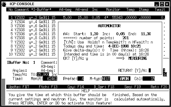
Determine the data collection time using the Automon feature. The appropriate monitor value is computed so that the current run will finish at a specified time. Automon is initiated by moving the cursor to the AMON field and pressing Enter. The screen shown in Figure 15 then appears.

  

Figure 15: Using Automon to compute a run length.

The number of days and the end time for the run are entered in the Automon page. Use 1 for delta-days if the run will go past midnight even if the run length is only a few hours. A run starting at 21:00 (9 pm) and ending at 9:00 (9 am) the next morning, would be entered as delta-days=1 and Time=9:00. The computed Monit value is set when Automon completes.

6.

Complete buffers for all the samples you want to measure. If many parameters are similar, it may be useful to duplicate the run information for other temperatures that you will wish to run. 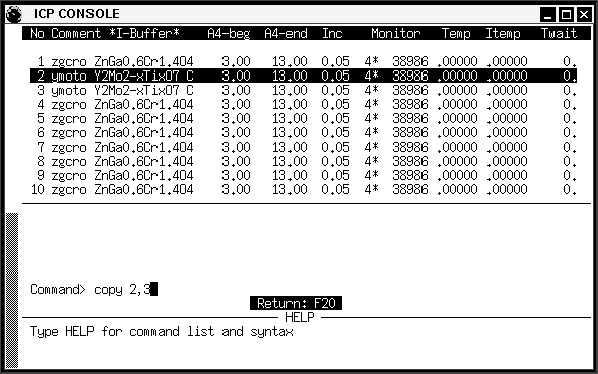This is done either by highlighting the buffer to be copied and then pressing the F14 key (actually the F6 key), which will copy the information to all other buffers, or (preferably) the buffer can be copied selectively by pressing the F18 key (actually F10) to enter the ``Buffer Ops'' mode where a buffer can be copied by entering a command such as COPY 2,3 (see Figure 16).

  

Figure 16: Copying a buffer in ``Buffer Ops'' mode.

This copies the parameters in buffer #2 into buffer #3. Exit ``Buffer Ops'' mode by pressing the F20 key (actually F12). Each buffer can then be quickly modified to change the appropriate fields.

7.

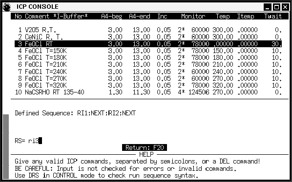
Once a series of runs has been defined, a ``run sequence'' can be defined by pressing the F19 key (actually the F11 key). This brings up the menu shown in Figure 17. If a previous sequence is present, it can be cleared by typing DEL and return.

  

Figure 17: Entering a ``Run Sequence'' for the sample changer.

Commands are added to the run sequence by typing RI#, where # is the buffer number of the run in the list. Commands may be entered one a time or several commands may be entered at once, separated by semicolons (;). Be sure to use a NEXT command between each RI# command so that the sample changer will be advanced to the next sample. The run sequence RI1;NEXT;RI2;NEXT;RI3 buffer 1 to be collected and the sample changer will be advanced and buffer 2 will be collected. The sample changer will be advanced again and buffer 3 will be collected. To skip a sample position, two next commands can be used: RI1;NEXT;NEXT;RI3 and it is also possible to collect multiple data sets on a sample: RI1;RI1;NEXT;RI2;NEXT;RI3. Exit the RS menu with the F20 key (actually F12).

8.

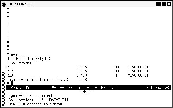
Switch to control mode by pressing the F17 (actually F9) key. The length of a run sequence can be estimated using the HOWLONG/RS command (see Figure 18).

  

Figure 18: Using the HOWLONG/RS command to determine the expected run time for a ``run sequence.''

9.

Before starting the run be sure to:

(a)

be sure the shutter is open

(b)

measure the monitor using the MRAT command

(c)

enter the sample composition and contact info on the white board

(d)

put the sample tag in the holder on the white board

(e)

enter the sample information in the log book.

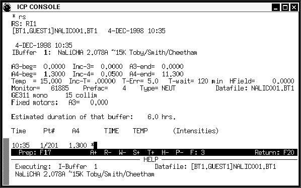
10.

The run sequence is started with a RS command, as shown in Figure 19.

  

Figure 19: Starting a ``run sequence'' with the RS command.

Note that it is possible to modify the run sequence or change the measurement parameters for the runs that have not been started in another (ExtraICP) window while the data collection is in progress.