 f24s>e
SEQfit option F,U,T,D,L,C,P,? Help or Exit :
f24s>e
SEQfit option F,U,T,D,L,C,P,? Help or Exit :
version 3.1, R. Ghosh, ILL, June 2001
This program uses the fitfun package to refine the starting parameters for fitting a sequence of diffraction patterns. A sequence of single or multiple pattern runs can then be analysed. Simple graphics are incorporated to enable the variation of derived peak parameters to be viewed and printed. An output file is created which can be read into a spreadsheet program like Excel.
In addition there is the possibility to normalise the initial data using a notionally flat pattern, e.q. typically measured from vanadium or plexiglass, either from a raw data file or a LAMP derived correction file.
The data sequence can be renormalised for a fixed incident flux by setting a proposed total flux monitor value. This helps in the analysis of kinetic data taken on non-linear time-scales.
setenv PGPLOT_DIR ../libm
setenv PGPLOT_ILL_DEV_1 /xserv
setenv PGPLOT_ILL_DEV_2 /VCPS
setenv PGPLOT_ILL_PPAGE 2

setenv D20_DATA_PATH /usr/illdata/data/d20/d20_0/
   (note the terminal "/")
  for data from 000001 to 009999
setenv D20_DATA_PATH /usr/illdata/data/d20/d20_1/
  for data from 010000 to 019999  etc.
The first four control the graphics, corresponding to X-terminal graphics, and PostScript output. The last concerns the location of the raw data files, and this may depend on the setup of individual workstations. If absent then the raw data are sought in the current directory.
If the data cannot be located, as a final resort you might try setting the source directory to the data fileserver with the following..
setenv D20_DATA_PATH /hosts/serdon/illdata/data/d20/d20_0/
or d20_1 etc as appropriate
For PC-Windows similar environment parameters may be set, or else combined in a batch file as shown below :
rem F24S.BAT
rem to ensure environment space is available launch this as follows
rem >COMMAND /E:2048 /C F24S.BAT
SET PGPLOT_ILL_DEV_1=/gw
SET PGPLOT_ILL_DEV_2=/VCPS
SET PGPLOT_ILL_PPAGE=2
SET PGPLOT_DIR=../libm
REM This directory contains font file GRFONT6.DAT
SET D20_DATA_PATH=C:\D20DATA (or wherever..)
REM to run program:
C:\FITD20\F24S  (or wherever the executable program is located)
Having set these initial values the C command continues treatment by using standard fitfun to read in data and set parameters by manual fitting.
Commands consist of one letter followed by either numerical input (free format) or a letter code (upper or lower case); fields should be separated by blanks or commas. Often the program would be used following the sequence given below.
R
The READIN routine is called after this command, and it makes a
new spectrum available to the fitting routine.
D
The current spectrum is plotted.
V
The current variable values are displayed. These are read initially
from a file named "pnam".ffn, where "pnam" is a four character name
defined in the MAIN routine. Parameter numbers 100, 200 and 300
control the fitting procedure (see below) and are not often
modified.
V n v s
The n th variable is set to the value v, and if it is to be fitted
the step s is set to 1. If the model seems very sensitive to this
parameter the value of the step should be reduced to .1 or smaller
and converse. It may be that the model algorithm should be recast.
Normally this should not be necessary. The variation of the n th
parameter can be constrained by being tied to a preceding parameter n'
if s is set to -n'.
X min max
If both min and max are absent or 0 the current spectrum scale limits
are displayed. These may be modified to the new values if these are
none-zero.
Y min max
See above - as for X scale.
F
Without an argument the fit with the current parameters is shown
together with the residual (sum of F(I)**2) normalised by the the
number of points. If the spectrum or fitting range is smaller than
the plotting limits and the Only option has selected a restricted
range then the calculated graph is extrapolated to the plot limits.
(First set the x axis limits, then set the O options). The difference
between the observed and calculated values are displayed offset with
zero at 80% of the yscale limits, with the same scale factors. Adjusting
the y-scale limits may be necessary to reduce overlap with the calculated
curve and data.
P
The fit as given above for F is written out into the second plotting
device defined. Usually this is a PostScript file.
F n [N]
Fitting is started with a maximum limit of n iterations. In general
this should be of the order m**2 where m parameters are being fitted
simultaneously. As fitting proceeds the step lengths for each
variable are also optimised. As a consequence giving a subsequent
F command to continue fitting further iterations resets the step
sizes, and the effect is different from giving a larger total
number initially. If the letter N is added then no intermediate plots will
be made.
L [F]
This produces a summary [or full listing] of the current fit on the terminal
and a file "pnam"xx.lis is produced which may be be printed after
leaving the program.
C
This toggles a cursor on or off for the next D, display command to allow the
current spectrum to be measured-up on-screen.
O a b c d e f
The spectrum is only fitted in the non-zero ranges:
a<x<b, c<x<d, e<x<f
The command O alone resets all points into the range to be fitted.
S
The current parameters are saved in the file f24s.ffn; this
permits an easy re-use for a subsequent analysis, or simply
to save current values while they are subject to delicate
manual adjustment. (Quit or interrupt program; then restarting will re-read
a saved "good"set of starting values!)
Z
This clears the plotting screen, useful in some terminal environments.
W name
The argument should contain five letters or numbers. The program writes out
the observed and calculated values into a file "name.fpl". The format
of this file is given in appendix 3.
J
The program calls a subroutine FTEXTP (a dummy routine is always
included in the library and is loaded when no personalised routine
is included). This enables the user to perform additional tasks,
e.g. in f24s, FIRR and TAPPIR component plots are made of separate
contributions to the resultant curve.
T text....
The additional text is placed on the following graphical output.
H
A summary of the above instructions is typed out. If the
programmer has himself provided a subroutine FTXHLP then this
replaces the dummy in the library, and offers a way of adding
further annotation on program use.
E
Exiting the manual stage of the program, having performed a
fit to the section of data, it is then possible to re-use the
peak parameters and steps to fit sets of data.
As for the fitfun layer the seqfit commands consist of one letter which may be followed by one or several numbers.
T run1 run2 sub1 sub2 [max-iterations] U run1 run2 sub1 sub2 [max-iterations] The T command will fit all data sequentially using the same starting parammeters. The U updates the parameters with those from the last fit. The run and subrun numbers may designate either an increasing or decreasing sequence. A maximum of 4000 fits can be performed in a 1 or 2 dimensional set of data designated by the run and subrun numbers. Normally the iteration limit of 100 is used by default. If treatment of an incorrect sequence of runs is accidentally started then typing [Control+C] will interrupt the data search sequence. Elsewhere this terminates the program.
L par1 par2 par3 par4.. After fitting the results for the sets can be shown by selecting the parameter numbers; up to 5 parameters and their standard deviations can be listed at each L command, and results are also sent to a listing file. Included too is the fit index, which is 0 when no problems have occurred, 1 when no minimum has been found (and the deviations are not reliable), and 2 when the iteration limit has been reached before them minimum.
D 1 (or 2) parameter-number
P 1 (or 2) parameter-number
D gives a summary plot of the selected parameter as a function
of run number (1), or subrun number (2) on the screen
(more explicitly the device defined in the environment variable
PGPLOT_ILL_DEV_1). P outputs the
results to a PostScript file (device defined in PGPLOT_ILL_DEV_2)
A text string
This adds the text string as annotation to the displayed data.
?
This command lists the numbers and names of parameters which have been
fitted.
H lists a summary of the sequence fitting commands.
% /home/cs/ghosh/d20/f24s
f24s - version 3.1 (R.E. Ghosh, ILL)
Fits up to 4 peaks in sequences of D20 datasets
Initial options to read and normalise subspectrum:
C Continue now to data fitting
V n Set vanadium run n
N name Set efficiency file name
M m Monitor renormalisation (o=none)
Z a modify zero angle (30.0)
L i j List run i subspectrum j
H Help
No vanadium normalisation run
Zero angle : 0.000
Efficiency file name Not used
New monitor value : 0.0
Type option C,V,Z,M,N,L,HELP : c
Fits up to 4 peaks in sequences of D20 datasets
Manual peak fitting and parameter initialisation
Peak type :
1 Single Gaussian
2 Single Lorenztian
3 Voigt - Lorenztian width shown
4 Skewed Gaussian
Modifier parameter for Voigt is Gaussian width
Modifier parameter for Skewed Gaussian is LHS-width/RHS
Width values are half width at half height
Background is value at centre of first peak
SEQfits v2.4 June 2001 (Ron Ghosh, ILL)
Prepare parameters for sequence fits by manually fitting some data
f24s version 3.1
TYPE HELP OR OPTION: H,R,D,X,Y,V,F,O,P,L,W,C,E,J,S,T,Z
f24s>r
Give run number...subspectrum number : 9201 1
THERE ARE 200 DATA POINTS IN CURRENT FITTING RANGE
TYPE HELP OR OPTION: H,R,D,X,Y,V,F,O,P,L,W,C,E,J,S,T,Z
f24s>d
TYPE HELP OR OPTION: H,R,D,X,Y,V,F,O,P,L,W,C,E,J,S,T,Z
f24s>v
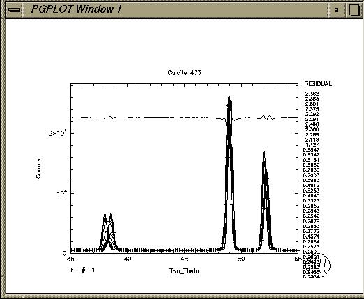
FITFUN 6.6 TITLE:Calcite 433
FITTING Y : Counts VERSUS X : Two_Theta
NUMBER PARAMETER VALUE ( OLD VALUE ) STEP % DEVIATION
1 FLAT BGD 550.0 ( 550.0 ) 1.000 0.00
2 slope BG 0.0000E+00( 0.0000E+00) 0.0000E+00 0.00
3 (spare) 0.0000E+00( 0.0000E+00) 0.0000E+00 0.00
4 FACTOR F 0.0000E+00( 0.0000E+00) 0.0000E+00 0.00
5 P1 type 1.000 ( 1.000 ) 0.0000E+00 0.00
6 P1 area 3000. ( 3000. ) 10.00 0.00
7 P1 width 0.2500 ( 0.2500 ) 1.000 0.00
8 P1 posn 36.00 ( 36.00 ) 0.1000 0.00
9 P1 modif 0.0000E+00( 0.0000E+00) 0.0000E+00 0.00
10 P2 type 1.000 ( 1.000 ) 0.0000E+00 0.00
11 P2 area 0.1200E+05( 0.1200E+05) 50.00 0.00
12 P2 width 0.2200 ( 0.2200 ) 1.000 0.00
13 P2 posn 49.00 ( 49.00 ) 0.1000 0.00
14 P2 modif 0.0000E+00( 0.0000E+00) 0.0000E+00 0.00
15 P3 type 1.000 ( 1.000 ) 0.0000E+00 0.00
16 P3 area 6600. ( 6600. ) 10.00 0.00
17 P3 width 0.2000 ( 0.2000 ) 1.000 0.00
18 P3 posn 52.00 ( 52.00 ) 0.1000 0.00
19 P3 modif 0.0000E+00( 0.0000E+00) 0.0000E+00 0.00
20 P4 type 0.0000E+00( 0.0000E+00) 0.0000E+00 0.00
21 P4 area 0.0000E+00( 0.0000E+00) 0.0000E+00 0.00
22 P4 width 0.0000E+00( 0.0000E+00) 0.0000E+00 0.00
23 P4 posn 0.0000E+00( 0.0000E+00) 0.0000E+00 0.00
24 P4 modif 0.0000E+00( 0.0000E+00) 0.0000E+00 0.00
100 MAXIMUM STEP 100.0 300 SUBSTEP 0.01000
200 ACCURACY 0.1000E-01
THERE ARE 200 POINTS IN THE CURRENT RANGE SET BY "ONLY" COMMAND.
CURRENT LIMITS (IF RANGE IS NON-ZERO) ARE :
35.0 TO 55.0 0.000E+00 TO 0.000E+00 0.000E+00 TO 0.000E+00
TYPE HELP OR OPTION: H,R,D,X,Y,V,F,O,P,L,W,C,E,J,S,T,Z
f24s>v 8 38 .1
f24s>s
TYPE HELP OR OPTION: H,R,D,X,Y,V,F,O,P,L,W,C,E,J,S,T,Z
f24s>f 100
FITTING.....
.....ENDED
TYPE HELP OR OPTION: H,R,D,X,Y,V,F,O,P,L,W,C,E,J,S,T,Z
f24s>e
SEQfit option F,U,T,D,L,C,P,? Help or Exit :
On starting the program offers a choice of correction methods to correct
for the detector efficiency, either a prepared calibration file
or a flat spectrum, e.g. vanadium. This section will also print
out any subspectrum of any run. It also allows the default zero
angle to be modified, and the data to be rescaled with an
alternative monitor value. Once satisfied the e command
exits this section and a manual fit to one spectrum must
be made to initialise the fitting parameters.
The pattern is read-in using the R command.
The fitfun package offers a D (display option) to view the input data and cursors/scale settings etc. as well as the ability to trial fit the data manually, and with a number of automatic iterations.
The current parameters are listed with the V command.
In the above example the first peak postion is adjusted to start with the value 38.0, and step finely with 0.1 * the nominal step (variable number 300 SUBSTEP) , since the fit is very sensitive to the position because the peak is very close to Gaussian, and well defined. Note that the step for the areas is set fairly coarsely; only approximate values are given. The parameters can be saved with the S command. As can be seen here only a range from 35 to 55 dgrees is being fitted, limited by the O command in a previous test, restricting the fit to 3 peaks only.
The current variables are saved with the S command manually. These will be reread should the program be interrupted and restarted.
The fit is then started limiting the number of iterations to a maximum of 100.
When the fit terminates these parameters can be transferred to the sequence treatment by exiting E from this manual phase. The results are stored temporarily.
The sequnce fitting options now appear and a sequence of runs and subpatterns may then be treated with the T or U command depending on whether the starting parameters are to be reinitialised or not. The program will treat ascending or descending series, to allow the best, but disappearing, peaks to be used to set the initial search state. When fitting becomes progressively more difficult certain parameters, notably the position, should be held fixed (step 0.0) which will limit the program from diverging when the peak is really difficult to resolve distinctly.
SEQfit option F,U,T,D,L,C,P,?, Help or Exit : h
SEQfits v2.4 April 2001 (Ron Ghosh, ILL)
Options:
F Fit one spectrum (manual fitfun)
+ other options - plots/cursor etc
U i j k l Treat a set of runs i to j
and subrun indexes k to l
Updating parameters
T i j k l Treat a set of runs i to j
and subrun indexes k to l
(re-use initial fitfun parameters)
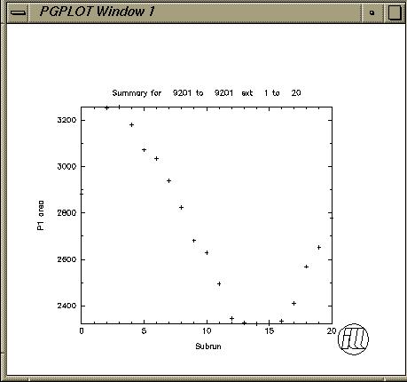
D 1(2) q [y0 y1] Display parameter #q results
for runs (1), subruns(2)
y-scale set between y0 and y1
L p q r.. List sequence results
C Cursor for next plot (toggle)
P 1(2) q [y0 y1] PostScript file of seq. plot
A text Annotate with text string
? show which parameters are fitted
H for this help
E Exit
SEQfit option F,U,T,D,L,C,P,?, Help or Exit : t 9201 9201 1 20
Run 9201 subrun 8 no minimum found
SEQfit option F,U,T,D,L,C,P,?, Help or Exit : ?
Fitting
Parameter number Name
1 FLAT BGD
6 P1 area
7 P1 width
8 P1 posn
11 P2 area
12 P2 width
16 P3 area
17 P3 width
18 P3 posn
SEQfit option F,U,T,D,L,C,P,?, Help or Exit : l 1 6 7 8
run ext Backgr % P1 area % P1 width % P1 posn % fit_fail
9201 1 557.8 1.0 3256.0 1.76 0.261 1.65 38.53 0.01 0
9201 1 557.8 1.0 13097.3 0.81 0.228 0.69 48.89 0.00 0
9201 1 557.8 1.0 6597.9 1.18 0.247 1.05 52.21 0.01 0
9201 2 557.7 0.9 3260.7 1.61 0.260 1.51 38.52 0.01 0
9201 2 557.7 0.9 13067.3 0.74 0.229 0.63 48.89 0.00 0
9201 2 557.7 0.9 6328.9 1.06 0.249 0.95 52.21 0.00 0
9201 3 556.3 0.9 3183.3 1.68 0.260 1.55 38.53 0.01 0
9201 3 556.3 0.9 12830.1 0.78 0.229 0.66 48.89 0.00 0
9201 3 556.3 0.9 6155.3 1.10 0.252 1.01 52.21 0.00 0
9201 4 555.6 0.9 3071.6 1.62 0.260 1.50 38.53 0.01 0
9201 4 555.6 0.9 12607.0 0.75 0.231 0.65 48.89 0.00 0
9201 4 555.6 0.9 5922.5 1.05 0.252 1.02 52.21 0.00 0
9201 5 553.8 0.8 3037.7 1.52 0.263 1.54 38.53 0.01 0
9201 5 553.8 0.8 12366.1 0.70 0.232 0.68 48.90 0.00 0
9201 5 553.8 0.8 5622.0 0.97 0.254 1.05 52.21 0.01 0
:
:
SEQfit option F,U,T,D,L,C,P,?, Help or Exit : d 2 6
SEQfit option F,U,T,D,L,C,P,?, Help or Exit : p 2 6
SEQfit option F,U,T,D,L,C,P,?, Help or Exit : e
Closing listing file f24s294.lis
Closing output result file f24s293.sls
%PGPLOT, Closing file f24s292.ps
The final column contains a fit result. Usually this is 0, indicating that a minimum has been found without any problems. When set to 1 the final fit may not be the absolute minimum because the step sizes are typically too small for peak areas, or too large for positions. The manual fitfun option F can be used to modify this, or to examine the fit for any individual component, by opening that data file going back into fitfun F, and selecting the subspectrum in doubt, and reperforming the fit.
Feedback on this program will be welcomed by the author, Ron Ghosh reghosh (at) gmail.com