Once the center of the diffraction arcs has been determined and the background has been subtracted you are ready to generate a synthetic digital diffractogram. I'm going to work from here in Image J since it is fast and easy to use.
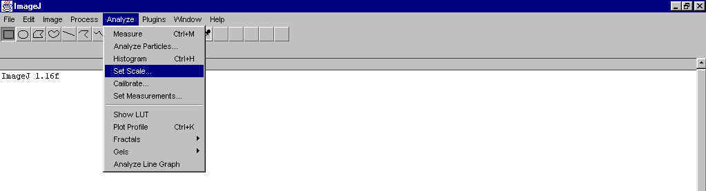
The first step is to set the scale
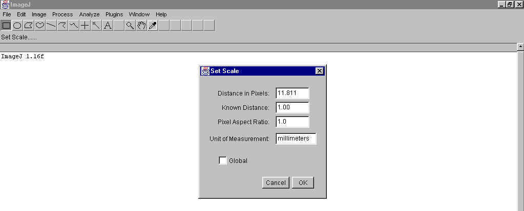
The Set Scale window will appear. The Distance in Pixels box will have some arbitrary value entered in it. Change this to the number of pixels per millimeter that matches the DPI of your scan. I've shown 11.811 which is for a 300 DPI scan (300/25.4 = 11.811 pixels per millimeter). Check that the Unit of Measurement box is changed to read millimeters instead of the default "inches"
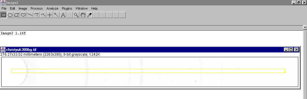
Open the background subtracted image and using the rectangular ROI tool draw a long narrow box with one end directly on top of the centering mark and with the box straddling the center line of the diffraction pattern. An example of this ROI is shown below.
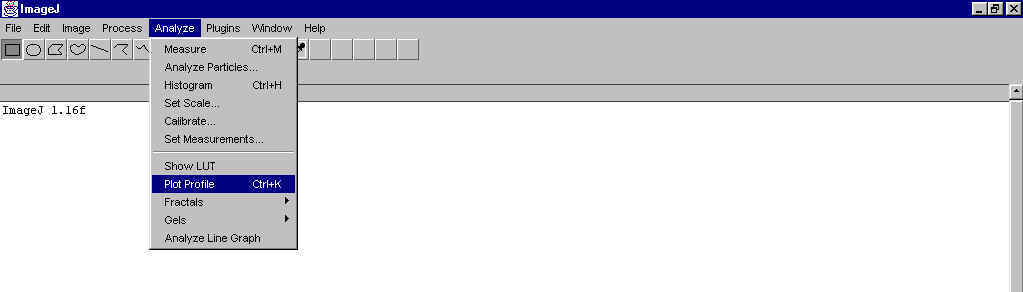
Once scale has been set and the ROI has been drawn, you are ready to generate the diffractogram. Under Analyze, select the Plot Profile function.
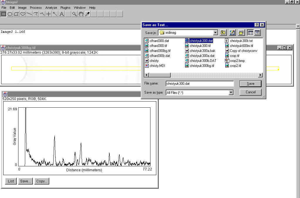
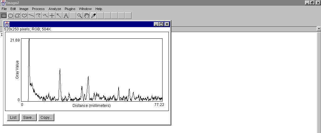
The plot will generate a diffraction pattern calibrated in millimeters with the zero point corresponding to the center of the diffraction arcs. The quality of the diffraction pattern will depend on the original film, the scan quality and the precision of measuring the center point. An example of the diffractogram (plotted profile) is shown below.
In order to use the data set of XY values from the plotted profile you must first save these values. The saved output is an ASCII text file and can be saved as a *.DAT file for convenient recall into other programs. Note that ImageJ does not specify a file type and you must write out the filename and .DAT extension as in this example